What is this post?
This is a brief recap of my 1st presentation in class. This post will cover some of the technical details I presented on as well as serving as a place to leave comments.
Redux
Why curvature and why a torus?
The active nematic material we are working with is a soft material. This implies that it is easily deformed and thus sensitive to forces that hard materials can easily ignore. Macroscopic curvature is one of these forces. In fact, the connection between nematic order (specifically in thermotropic and lyotropic liquid crystals) and curvature is well-studied and actually lies at the heart of the free-energy typically used to evaluate nematic configurations.
We are looking at active nematics on the surface of a torus becuase the torus gives us an opportunity to examine the effect of changing curvature. Unlike a sphere, the curvature on the surface of a torus changes depending on the location. For example, a torus will always have a smoothly varying Gaussian curvature between its maxmimum along the outer ring and its minimum along the inner ring. In addition, the maximum Gaussian curvature is always positive and the minimum Gaussian curvature is always negative.
How do we process the data?
In the last post, I chose the nematic order paramter, Q, a symmetric traceless rank-2 tensor, as the microstructure function. As a brief aside, we use a rank-2 tensor due to the head-tail symmetry of the nematic structure. If we tried to define a vector (rank-1 tensor) for the nematic, we would always find that the vector was 0.
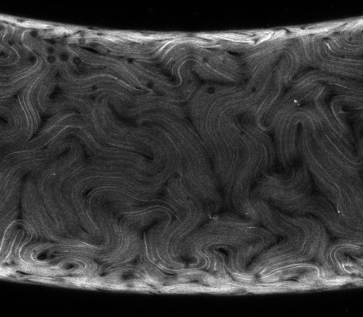
To determine Q everywhere in our data, we first use a technique called “Coherence-enhanced diffusion filtering.” The basic idea behind this technigue is to make an averaged rank-2 tensor from the gradient of the image intensity. From this “structure tensor”, we get the local orientation everywhere in the image. We then average over this local orientation to find Q. An example analysis showing how we move from the raw data to the microstructure function is below.
|
z-stack |
maximum intensity projection |
|
- First, we take our 3D (x,y,z) array of data and project it to a 2D (x,y) array by only keeping the maximum intensity along z for each (x,y) coordinate. Above, a video scanning through the 3D array along z is seen on the left and the maximum
|
gaussian-filtered image |
gradient orientation on the intervel [0 (black),180 (white)] degrees |
|
|
|
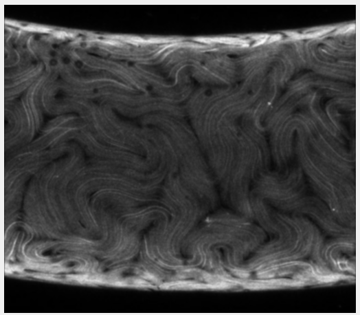

- We filter the maximum intensity projection with a Gaussian filter to denoise the image, as seen in the example above on the left. Then, we take the gradient of the denoised image and construct a symmetric tensor using the outer product of the gradient with itself. The orientation of the gradient folded over the interval [0 (black),180 (white)] degrees can be seen for the example above on the right. The orientation is measured CCW off of the horizontal.
|
local orientation on the intervel [0 (black),180 (white)] degrees |
|
|
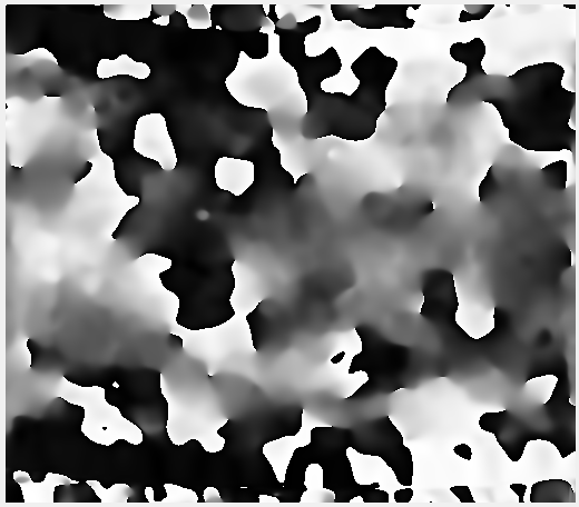
- To get the structure tensor we componentwise average the gradient tensor using a Gaussian filter. The standard deviation of this Gaussian filter should be about the size of the nematic features we want to characterize. The local orientation at every point is given by the eiqenvector associated with the smallest eigenvalue of the structure tensor at that point. An example local orientation image on the interval [0 (black),180 (white)] degrees measured CCW off of the horizontal can be seen above.
|
director orientation on the intervel [0 (black),180 (white)] degrees |
S on the intervel [0 (black),1 (white)] degrees |
|
|
|

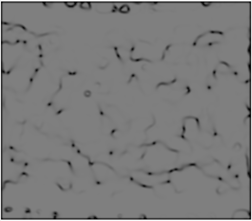
- Lastly, we average over this local orientation using a median disk filter to find Q for every point. We represent Q using two quantities, the director “n” and the degree of alignment “S”. These can be seen above for example analysis on the left and the right, respectively. The director oriention is displayed on the interval [0 (black),180 (white)] degrees measured CCW with respect to the horizontal.
This gives us a digital representation of our microstructure from our raw data,. Now that we have something to work with, we can construct the workflow for the data analysis and the remainder of the project…