2-Point Statistics Workflow:
Two-point statistics are going to be computed using the PyMKS framework developed in Python by the MINED group. The advantage of using this PyMKS code is its convenience in implementation and good support from the developer(s) of the code, David Brough, and others in the MINED group. Initial computations were done in Matlab framework, also developed by MINED. We have a three-phase structure, and essentially we have 0, 1, and 2 assigned to each phase. We assume a periodic structure, which is based on the boundary conditions of the simulation.
After computing the spatial statistics for one dataset, the next big challenge is determining a representative structure within the dataset. A representative structure is needed in order to simplify the data analysis further down the pipeline. For each dataset we expect to extract one set of spatial statistics. Since we have a three-phase structure, we have 6 spatial correlations total, 3 auto-correlations and 3 cross-correlations.
 Which microstructure can be chosen to represent all 4?
Number of computations
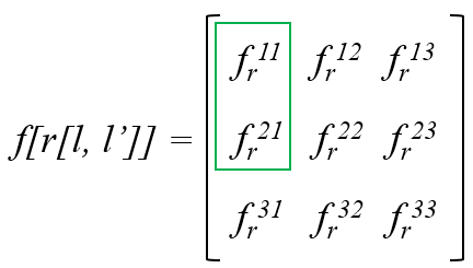
To obtain full spatial correlation for a three-phase material, we need to compute correlations on two statistics as shown below. There are 9 statistics total, of which three are redundant, for example statistics for indices ij and ji are the same.

In most of our datasets, there are about 300 structures. Initially, we compute the statistics for all structures within one dataset. Then, it’s possible to see trends and in the statistics to figure out the required frequency of computations.
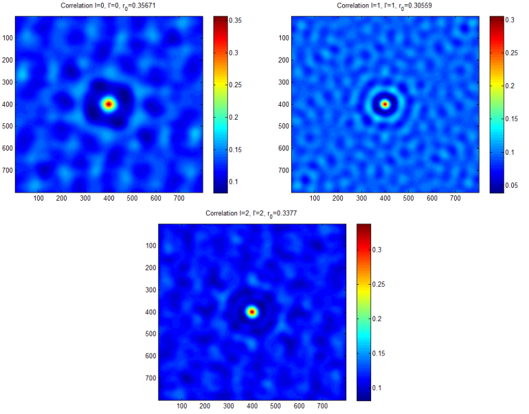
Example of auto-correlation is shown below:

Difference between statistics within a dataset
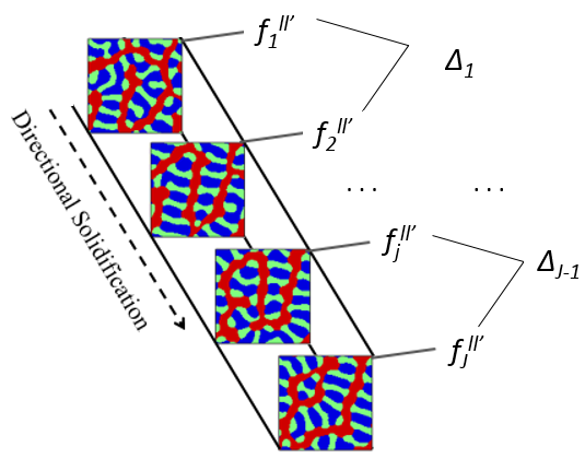
As the structure evolves with time and distance, we observe changes in the 2-pt statistics at each structure. To visualize how much each successive structure differs from the previous, we summed all the statistics within each structure and calculated the weighted difference. In J structures, we can extract J-1 weighted differences (delta) as shown below.

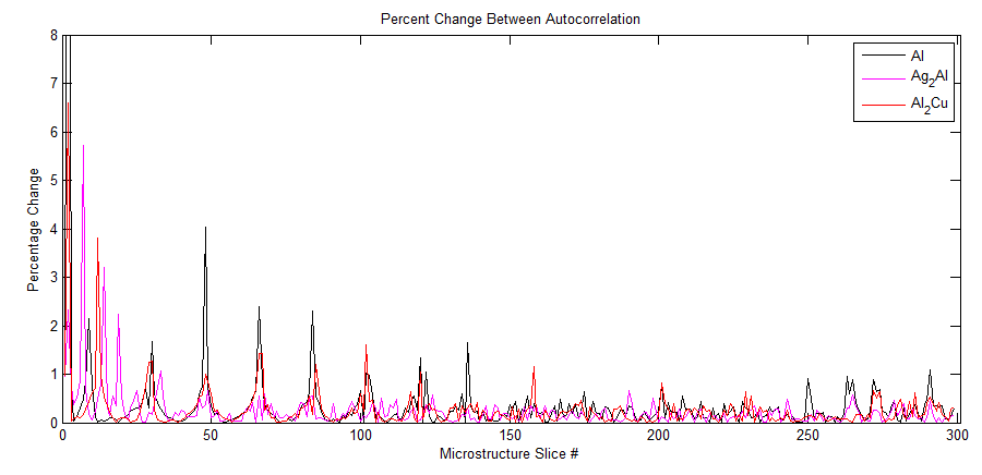
PLotting the deltas (autocorrelation for phases 0, 1, 2) between all microstructures, we can observe that initially the delta is very high (700%+). As the simulation continues, we see oscillations with lower amplitudes, which can be the beginning or the actual steady state of the structure. We also note a periodic pattern of the 2-pt statistics in the phases which is an interesting feature and could be something to look into in the near future. The represetntative structure could be chosen as the average of a selected steady-state region or a particular structure that is close of the same average.
 Note: y-axis is x100% percent
This is the preliminary method in obtaining a representation of the whole dataset. Other methods can include Representative Volume Element (RVE), or 2-pt statistics in 3-D space. Any suggestions are welcome!
Takeaways:
- Three-phase structure
- Periodic axes
- Representative structure: steady-state average, RVE, or another method.