Progress Report III (Post)

Posted by Almambet Iskakov, Robert Pienta on November 24, 2015

Quick Recap

Reduce our correlations to only the essential ✓
Truncate the 2-pt statistics ✓
Study our transient data ✓
Use time-varying regression to model our simulation data

steady

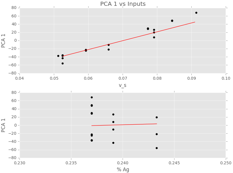
Reducing Correlations

Only two sets of correlations are dependent, clearly the model doesn’t need all six
This doesn’t mean all pairs of correlations will work equally!
We ran our entire pipeline on combinations of two correlations to see which perform the best
This was computationally expensive, but still feasible to do with just 6 choose 2 combinations.
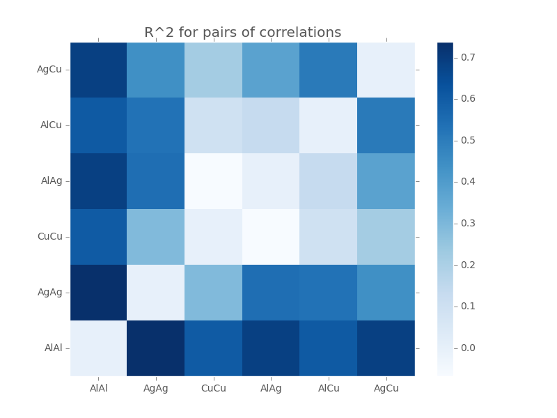
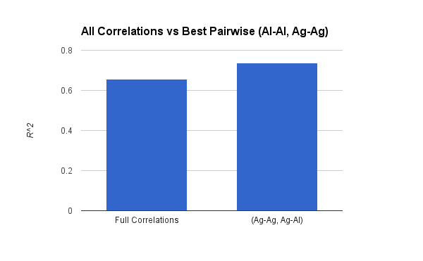
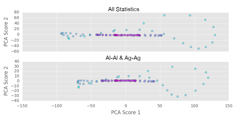
Ag-Ag and Al-Al performed the best with $r^2$ around 0.74
Al-Al and Ag-Cu performed very close with $r^2$ around 0.72

Truncating statistics

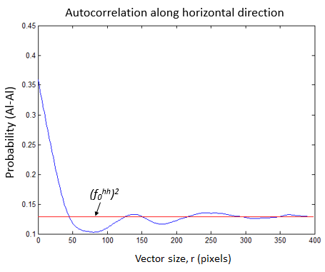
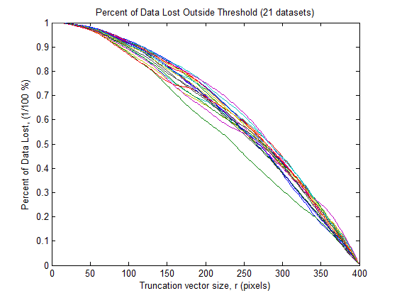
Truncation based of average 2-pt statistics in each sample in steady state

Al = Green, Ag₂Al = Orange, and Al₂Cu = Blue

Choosing a vector size

vector_size

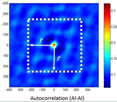
Example for autocorrelation

horizontal_auto

All steady state data

combined_violation

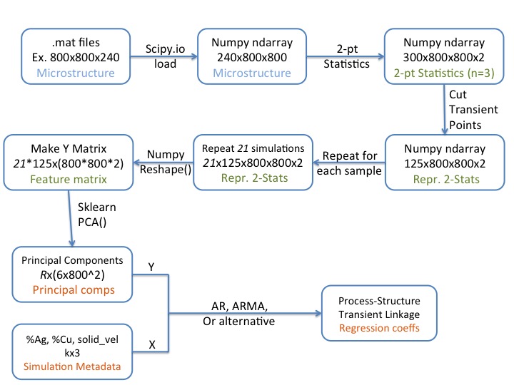
A New Pipeline

We created a whole new pipeline to perform our transient data linkages.
Its more than 100x more expensive than the previous pipeline

workwork

Transient Data

PCA components of a single simulation over time transient

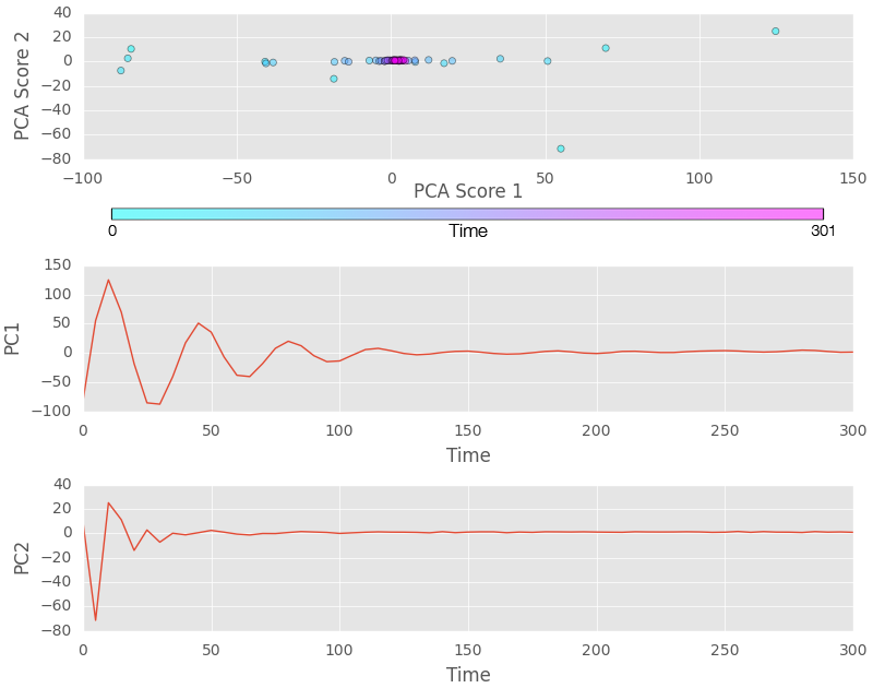
Wild oscillations until the early 100s

Here are just the first 100 points plotted out: transient

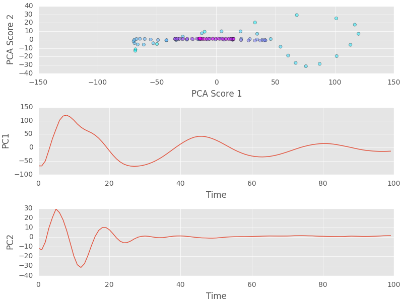
A sanity check of our correlation pair from earlier transient

Future Work

(Nov) modeling the time-varying behavior of our system (we are close!)
(Nov) post about transience
(Nov) post about steady state performance
(Dec) Final “In Summa” Post
(Dec) Final Presentation