This is the post equivalent of the presentation given for our first progress report.
Theory Outline
- Background Theory on Grain Growth
- Objective of our Project
- Intended Approach
- Input and Output Analysis
Theory on Grain Growth and Objective
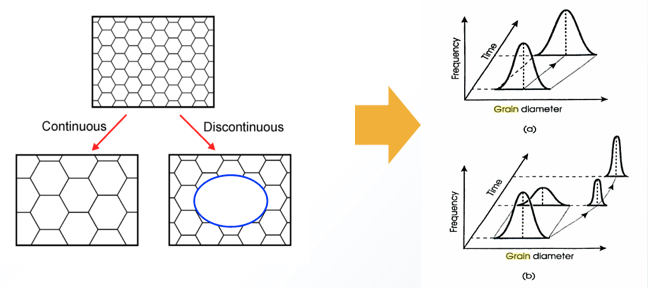
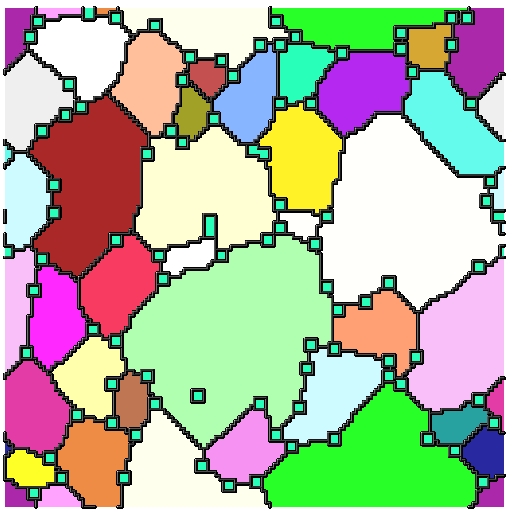
- The driving force for grain growth is the grain boundary interfacial free energy.
- Precipitates “pin”, deter, this grain growth since they reduce the surface area when a boundary crosses a precipitate.
Objective
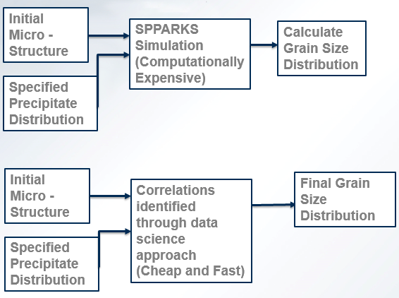
- We are using Kinetic Monte Carlo equations through the SPPARKS Program to analyze the effect of different precipitate distributions on the Grain Growth of a Microstructure and ultimately its size distribution.The process Spparks simulates is ageing.
- Then we want to predict with sufficient accuracy and in a computationally non-expensive fashion the correlation that exists between a specified Distribution of Particles and the Final Microstructure. This will be achieved by using a Data Science Approach.
- Thus we are establishing a Process-Structure Relationship
Inputs and Outputs
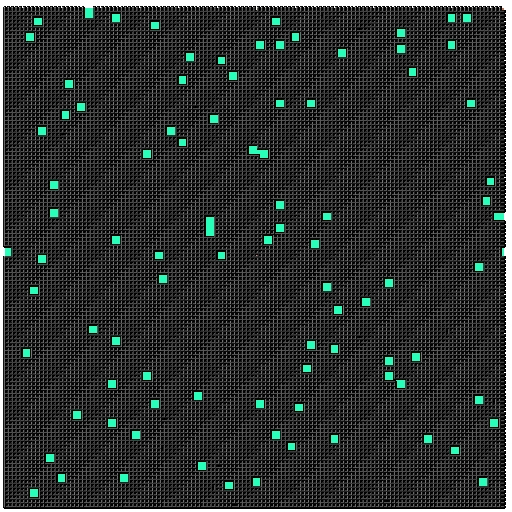
- We have an initial random Microstructure to which we are going to place various different distributions of precipitates.
- Random
- Uniform
- Clustered
- We will also vary the shape, size and volume fraction of Precipitates.
- Perform enough Simulations to have a enough statistical data.
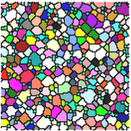
- On each simulation we can output various snapshots of the Micro Structure so we can calculate the grain size distribution and as well observe its evolution history.
Data Outline
- Data Tools and Generation Workflow
- How Much Data?
- What is the Data?
- Current Status
- What’s Next
Data Tools
- SPPARKS: open source code developed by Sandia National Labs
- PACE: computing cluster
- Pinning algorithm: allows pinning of different distributions
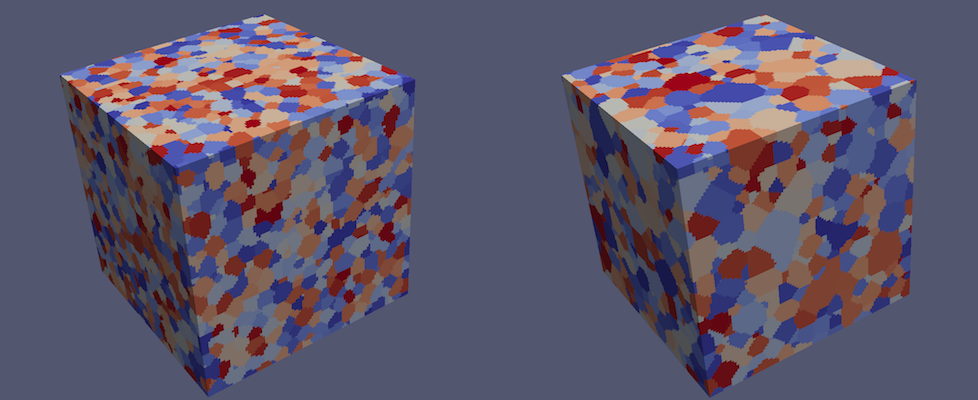
- Paraview: 3D visualization software
Data Generation Workflow
- Create initial/master random microstructure using SPPARKS
- Apply pinning algorithm with desired variables selected
- Run SPPARKS on PACE on our pinned microstructure to simulate grain growth
- View 3D models in Paraview
Goal: one button that does it all.
How Much Data?
We are varying 3 variables in our simulations
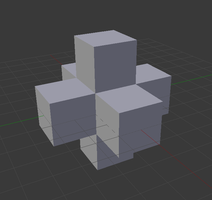
- Pin size/shape:
- 0 neighbor cube (single voxel, 1x1x1)
- 1 neighbor cube (3x3x3)
- 2x2x2 cube
- 2x1x1 prism
- 3x1x1 prism
- 3D plus sign
- Pin percentage: {0.5, 1.0, 1.5, 2.0, 2.5, 3.0}
- Pin distribution: random, uniform, cluster
How Much Data?
- Pin size/shape: 6 options
- Pin percentage: 6 options
- Pin distribution: 8 options
Total number of simulations to be run: 6 x 6 x 8 = 288
Note: this could be reduced depending on computational time!
What is the Data?
- Each microstructure is 300x300x300 voxels
- Full 3D data of pinned microstructures growing
- We have 300 images for a given time-step in the simulation
Current Status
- We have compiled SPPARKS on PACE and became familiar with running simulations
- Developed pinning algorithm for random and uniform distributions, missing clustering
- Able to successfully simulate grain growth with pins and visualize growth in 3D as animation/movie
What’s Next
- Finalize number of variables
- Patch tools together in master program that inputs our variables and outputs simulational data
- PyMKS and 2-point statistics — coming soon!