Model Recap
Recall we are building model to constructing process-structure linkages for pinning microstructures with precipitates and subjecting each sample to a grain growth process. For our model we have the following input and output:
Input: autocorrelation of pins with pins of multiple simulations.
Output: chord length distributions of the corresponding simulations.
PCA Output Problem and Fix
Our PCA code and coloring is ready to go and we’ve performed some analysis on the simulational data we already have. By plotting each average chord length distribution as a single point in PCA space, we were hoping to see some some of trend as a path or cluster. Turns out we saw more of a point cloud, which is neither of those trends. An image depicting that is below.
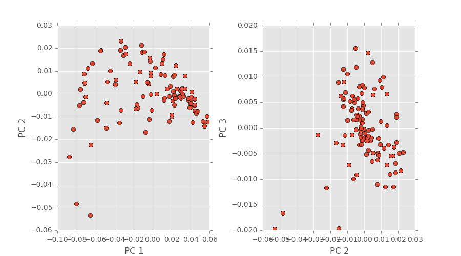
After some further inspection (read: time-consuming reverse engineering), turns out our segmentation code had a small error in the computation. After finding this we decided to do image segmentation differently and David has already made the change and shown new, promising results. We’ll update once the new plots have been made.
PCA Input Memory Problem Fixed
You might remember that our 3D simulations are rather larger: 300x300x300. So when performing PCA on the autocorrelations of the pins and pins we get a data matrix that is of size (n_simulations,27000000). That’s a big, dense matrix too. PCA on a dense matrix of that size is not easy on the memory of a computer. In fact, I’ve overloaded the memory on my MacBook Pro many times during the past two weeks working on this part of the project.
We discovered that PyMKS is storing some extra copies of the statistical data, which was eating up too much memory. We switched over to Matlab in the hopes of discovering the memory problem wouldn’t be as bad, even if the computational time was longer.
Good news: I was able to do PCA on a (108,27000000) matrix on 16GB of ram on PACE in ~40 minutes. It’s not the best thing in the world, but it’s better than nothing at all. Now that we know our input basis can be calculated and scaled even bigger things are looking good. Below is a plot of of 108 simulations and their autocorrelations described above.
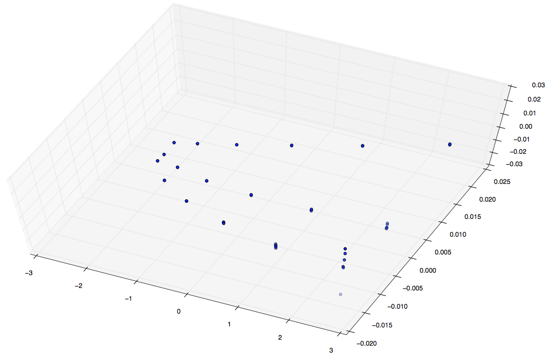
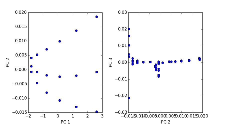
The first image is a 3D plot of the points. The second is a projection onto PC1,2 and PC2,3. A few interesting characteristics about these plots:
- Notice the three paths illustrated. These represent each pin shape, since of these 108 simulations we only varied our shape between three classes.
- In each path there are six data points (clusters). These correspond to the six percentages we varied in shown 108 simulations.
- Notice for each of the six data point clusters there are size points each. Since these pins are placed randomly we ran each simulation 6 six times to capture some more variance and cover out domain space better.
It’s interesting to see that 2 point statistics can point out commonalities and correlations even between randomly distributed pins/pixels. Keep an eye out for more plots soon!