Why do we need this equation?
Our first step in the reconstruction problem is to generate the 2-points statistics from the SAXS images. To do that we need to find the equation that links the electron density to the autocorrelation function.
The next image shows what happens theoritically.
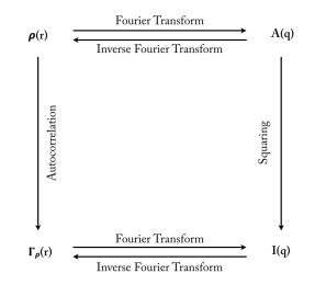
where $ \rho(r)$ is the scattering lenght density distribution A(q) the normalized amplitude of scattering I(q) the scattering intensity $\Gamma_ \rho(r) $ the autocorrelation function
The first path $\rho(r)$ to A(q) (just a FT) and then to I(q) ( the squaring) is the basic transformation behind Xray scattering and it’s non reversible. We loose the phase information following this path, reason why it’s impossible to reconstruct the initial microstructure by following the inverse path.
The second path $\rho(r)$ to $\Gamma_ \rho(r) $ and the I(q) is non unique. It is entirely plausible for the experimental scattering to be accurately described by a multiple of hypothesized $\rho(r)$.
So the only way to reconstruct the microstructure is to follow this path: 1. From I(q) calculate the 2-points statistics autocorrelation functions 2. Apply a phase recovery algorithm 3. Reconstruct the possible microstructures
Relation between the 2-point statistics and the scattering intensity
To solve the first point on our project, we need to derive the auto correlation of a local state from the scattering intensity. This derivation equation was already solved by David Brough. For more details on how it was done follow the previous link. Here is final equation to obtain the autocorrelation of phase 1.
Let know clearly define each components of this equation.
- We will be using the SAXS images for the reconstruction, so our microstructure function will have 2 local states: amorphous region and crystalline region.
- The scattering intensity is already known I(q) from the SAXS
- $ V_1 $ is the volume fraction of local state one. For each sample we have the percentage of crystallinity. So the volume fraction of crystalline and amorphous regions is known.
- For the quantity $V \eta_o^2 $ we need to develop the math a bit more to undersatand how to find it.
SAXS data provides the difference in electron density in the range of 1 to 1,000 nm. This difference can be represented as deviation from the mean electron density, $ρ¯$ as shown below.
$\eta(z)$=$ρ(z)$-$ρ¯$
We can show that $\Gamma_ \eta $(0) =$V \eta_o^2 $ (see derivation)
Then let consider the the quantity Q define by: Q=$\int I(s)ds$, Q is the sum of the intensity of our scattering volume (the total scattering power of the specimen).
$Q= \int \Gamma_ \eta(r)[\frac{1}{(2\Pi)^3}\int e^{-ikr} dk]dr $=$ \int \Gamma_ \eta(r) \delta(r)dr$= $\Gamma_ \eta $(0)
So Q=$\Gamma_ \eta $(0)=$V \eta_o^2 $
So our problem becomes easier to compute
where Q is the sum of the intensity
Sources
[1] R. J. Roe, Methods of X-Ray and Neutron Scattering in Polymer Science, 174-176, Oxford University Press 2000.