Review
Remember that we have decided to update our process to use the localization process in pyMKS formerly known as the MKS method. The predictions of the full strain tensor will be necessary to predict the damage caused by multiaxial loadings.
Prediction Procedure
The training to predict multiaxial loading conditions requires training for each of the tensor components.
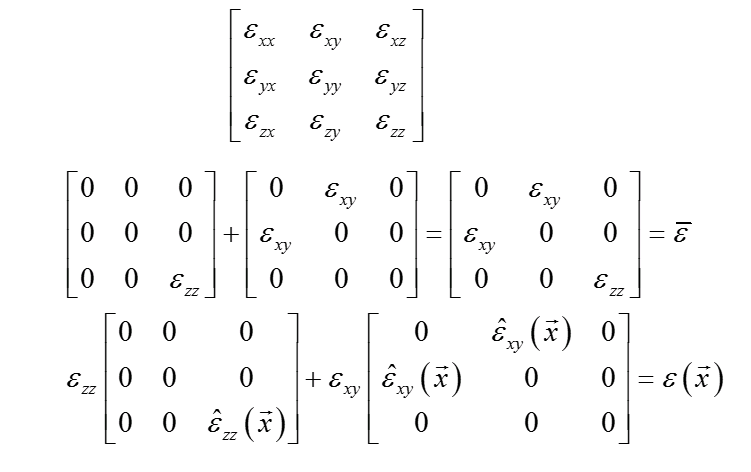
Since the material behavior is assumed to be linear-elastic for the MKS training, the overall response can be created by superposition from the individual component responses.
This is represented in the second line with the overall macroscopic response as $\overline{\varepsilon}$. The training is performed on the 6 tensor components by keeping the other components fixed and applying a known macroscropic deformation to the training component. The influence coefficients are then normalized by the known applied loading.
The third line shows the application of the superposition to the prediction of the localized response. The $\hat{\varepsilon}$ are the predictions from the normalized MKS influence coefficients. These predictions are then scaled by the imposed macroscopic load to predict the full localized tensor.
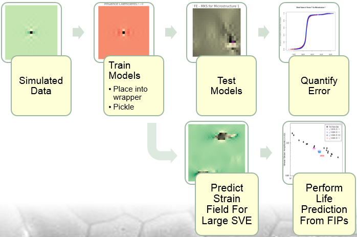
Overall Pipeline
The simulated training data consists of 21x21x21 delta microstructures. This size was chosen to reflect the relative inter-particle spacing in the region of interest (the “stringer” spacing based on a resolution of .5 um).
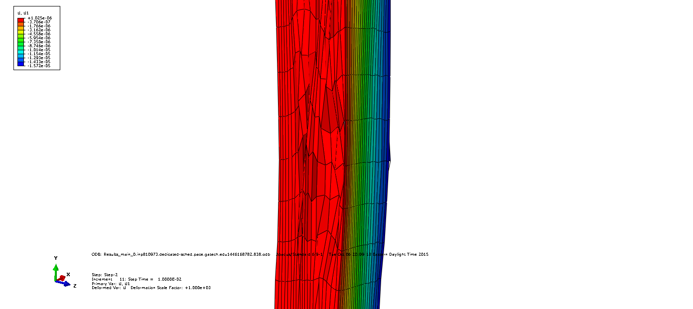
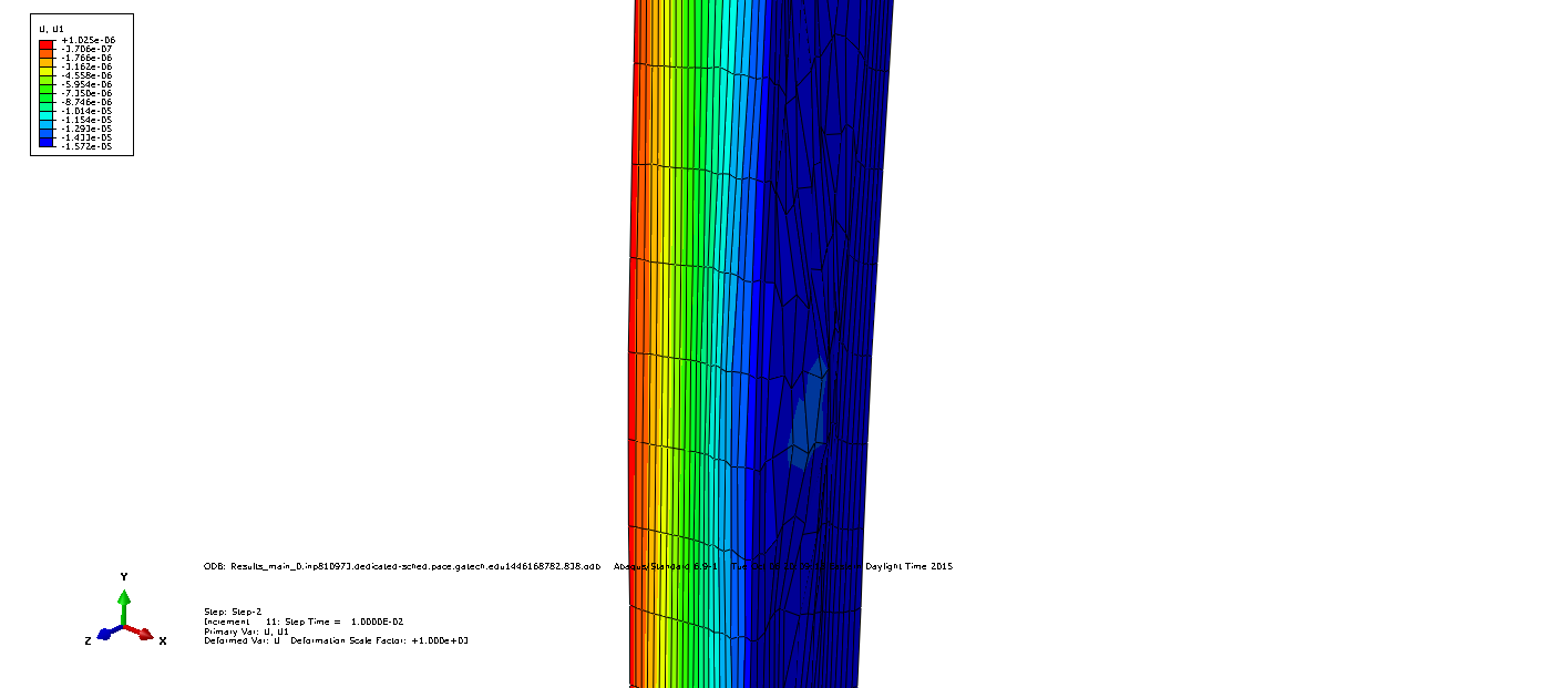
Periodic boundary conditions are applied. Since strain is the quantity under investigation constraint equations take the form
$L_i$ are the sidelengths $u1_j$ and $u2_j$ are the displacements in the respective directions. An example of exaggerated displacements can be found below for opposing faces.
The testing that has previously been mentioned with error analysis has been performed without any scaling of the influence coefficients (replicating the same macroscopic loading conditions for training and testing). Later posts will address the combined loading predictions.
The calibration of influence coefficients is performed directly from the crystal plasticity model that has been calibrated in previous efforts of the McDowell lab to model Al 7075-T6. Once the influence coefficients have been calibrated, they can be saved using the cPickle module in Python, saving us the effort in recalibrating every time a prediction must be made.