What is this post?
This is a brief recap of my 2nd presentation in class. This post will cover some of the technical details I presented on as well as serving as a place to leave comments. In addition, I will go over some of the relevant things that have changed since the presentation.
Redux
Where are we?
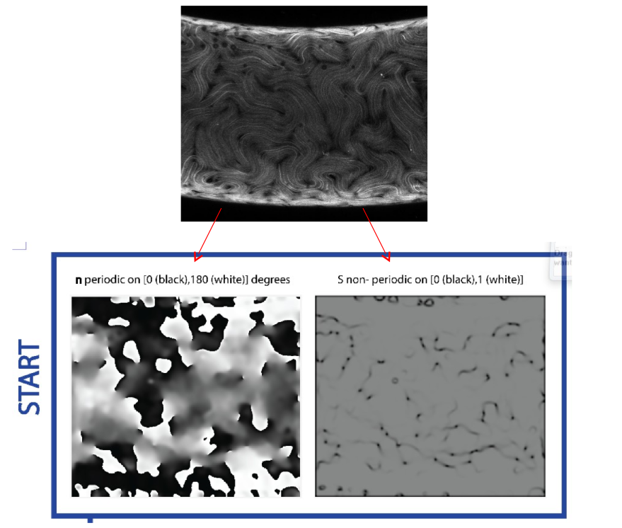
From some earlier posts, we established how to get from our 3D data to a 2D projection, and then how to get from a 2D projection to a description of the nematic order paramter Q for the entire projection. Below is an original data image and with arrows pointing to its Q and S values.
What needs to happen to run statistics?
From our workflow, the next steps are to (1) sort the data into bins where each bin has the same Gaussian curvature “width”, (2) sample the data in each bin using the same sampling length, (3) recast the director n in terms of a Fourier basis (because the data are periodic) and recast the degree of alignment S in terms of the Legendre polynomials (because the data are continuous and non-periodic on the interval [0,1]), (4) take the outer product between n and S at each point to get the final microstate. Note that because we bin the images based on Gaussian curvature, the physical pixel width of each bin is not the same. This is the reason we need to sample the data as opposed to just running the statistics on the images directly.
Unwrapping the images
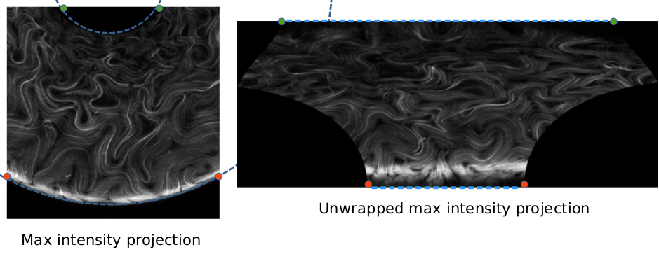
Looking at the original data image above, the lines of constant Gaussian curvature correspond to curves in the image that have constant distance from the inner and outer rings of the torus. For example, the uppermost curve in the image is the inner ring of the torus and the curve has the minimum (most negative) Gaussian curvature in the torus. In contrast, the lowermost curve in the image is the outer ring of the torus and the curve has the maximum (most positive) Gaussian curvature in the torus. By extention, the curve that is equidistant from the inner and outer rings of the torus will have zero Gaussian curvature. Thus, to bin the images, we must divide the image along these curves. Since this is difficult, what we will do instead is “unwrap” the image using the zero Gaussian curvature contour. Then, the rows of the unwrapped images will be the lines of constant Gaussian curvature and the binning process becomes trivial. In the example images below, an original data image (left) and its unwrapped counterpart (right) are shown. We have included some reference lines and points to show how the transformation affects the image, i.e. the green and orange dots represent the boundaries of the inner and outer rings of the torus, respectively in both images. The blue dashed lines show how the contours of constant Gaussian curvature in the original image becomre rows in the unwrapped image.
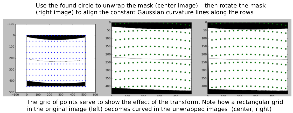
We perform the unwrapping process in python using a scikit-image function called PiecewiseAffineTransform. We perform the unwrapping using the circle found from the zero Gaussian curvature contour. This contour can be seen below using a mask.
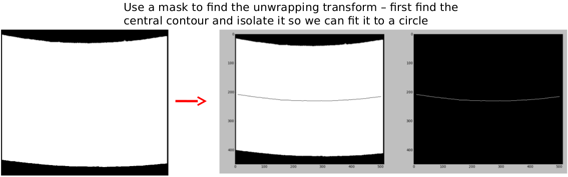
Once the image is unwrapped, we rotate the unwrapped image so that the straight lines representing constant Gaussian curvature align along the rows, as seen below. The grid points in the images correspond to each other and serve to show the effect of the transformation.
Binning the images
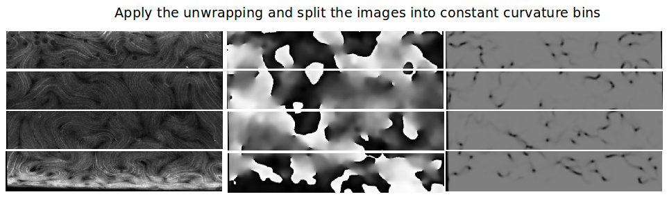
Next, we solve for the Gaussian curvature everywhere and split each image into “bins” of constant Gaussian curvature width. This is seen below for an unwrapped (left) original data image, (center) n image, and (right) S image.
What has changed for these steps since the presentation?
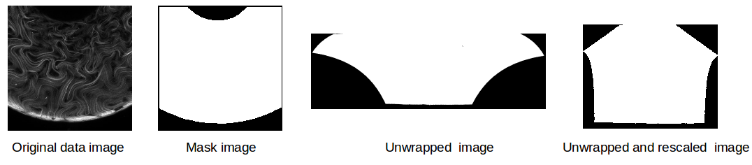
We have changed the unwrapping process to use MATLAB code instead of Python. This is purely a style choice as I’m much better in MATLAB and I didn’t have the time to properly debug the unwrapping function in Python (we were having problems for toroids with large Gaussian curvatures). In addition, we scaled all of the images so that every image has 1 px = 2 microns, regardless of the torus size or region shown. This makes the sampling easier. Below I show some mask images demonstrating the unwrapping and rescaling process for some mask images from a torus with large Gaussian curvature.