What is this post?
This will cover some of the issues we’re having with the statistics, show some (very) preliminary PCA, and outline what we want from this project and how we are going to move towards this in the month of November
What do we pass to PyMKS?
We pass the unwrapped and homoginezed n and S images, a mask for each image, a Gaussian curavture that defines the width of the bins, and some parameters that let us calculate the Gaussian curvature at each point (so we can bin the images propoerly). As an example, there are 74 images for torus D1. Each image has a scale of 1 px = 2 microns. Torus D1 has a ring radius of 283 px and a tube radius of 175 px. This means that a Gaussian curvature of produces 23 bins with px width from 3 px to 70 px.
What does PyMKS do?
PyMKS takes the stack of n (or S) images, bins the images, and creates a stack where the first 74 images elements are the sections from D1 from bin 1, etc. PyMKS then discretizes the images using a Fourier basis (or a Legendre basis for the S image stack) and then runs all the 2-pt statistics. Recall that our microstate for each point is really a multiple of n and S at that point. While we could do this mulplication before running statistics, we choose to do it after. This only works because n and S are independent. Once the statistics are run, they are stored in a list of lists, as:
Z x A x B x C x Stats
*Z = (statistics, category list) *A = Z[0] = (Legendre basis stats, Fourier basis stats) *B = (curvature bins) *C = (sliced image portion in the curvature bin in order D1_1 …D1_f,D2_1,…,D2_g,D3_1…D3_h) *Stats = numpy array with format (px width of bin x px length of bin x number of correlations)
This list is then saved to a pickle file.
What does the PCA routine do?
Since the px width of the bins can be small for some of the really negative Gaussian curvature bins, the PCA routine first only looks at bins with more than a specified number of pixels. This is so we can compare toroids with a large Gaussian curvature range against toroids with a small Gaussian curvature range. Then the n statistics and S statistics are multiplied against each other. The last step before performing the actual PCA is to form the giant array holding all of the statistics. This is done using by reshaping and flattening the list of lists. Finally, this giant array is passed to the scikit PCA routine.
Example stats
Below are some example stats for n represented using a Fourier basis. Even though I’m ostensibly showing the constant component term on the far left, note the “bands” in the statistics. This could means that something went wrong at some point as the bands can be a signiture of a machine error. David Brough is looking into this farther and we hope to have it resolved soon.
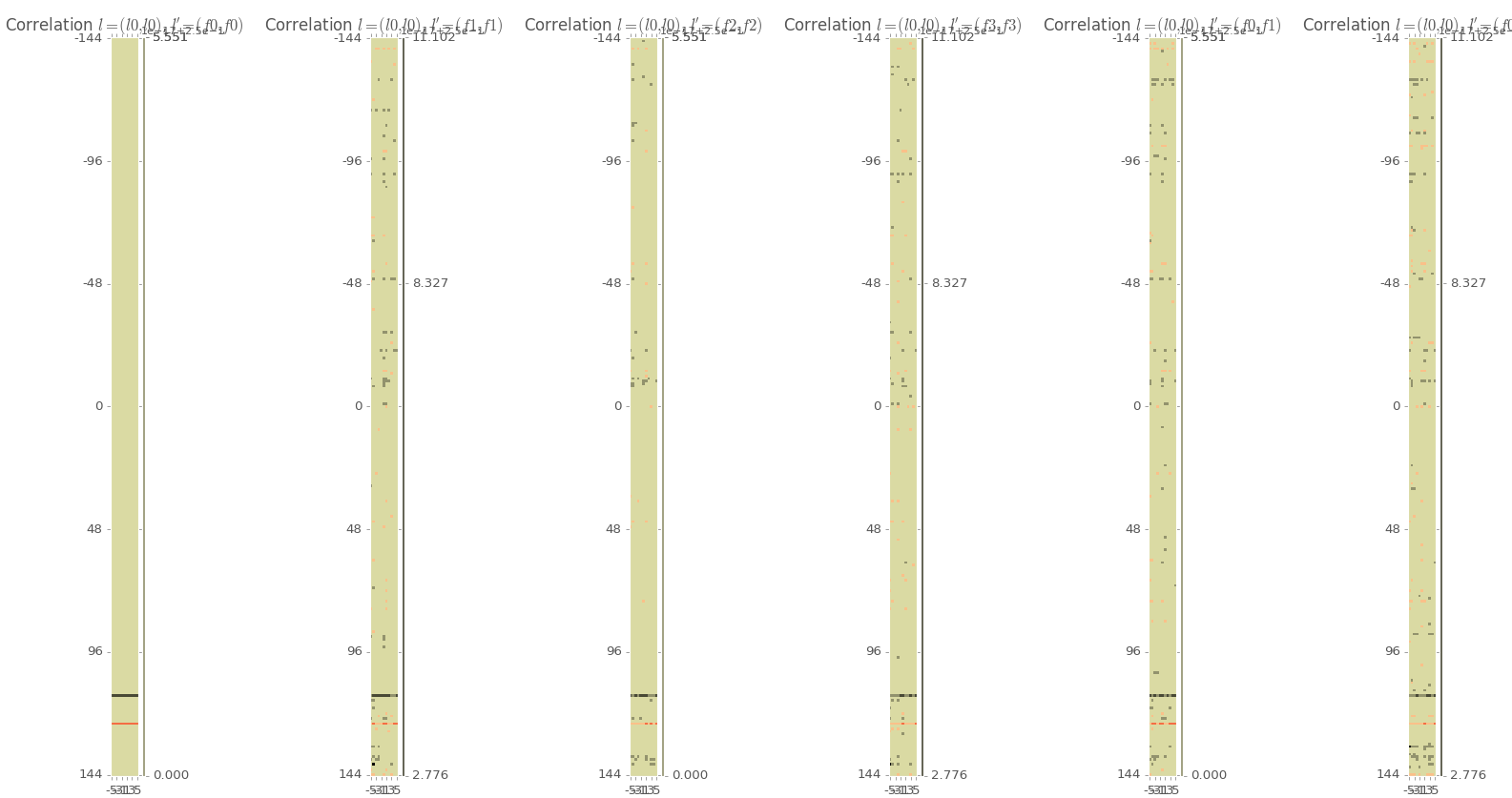
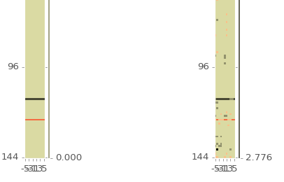
All stats are showing the constant component of the Legendre polynomials multiplied with the (from left to right) autocorrelations for the 0,1,2,3 Fourier terms, the crosscorrelation betweeon 0 and 1 Fourier term, and the crosscorrelation between the 0 and 2 Fourier term. Note the bands in the lower left of the left 2 images. A zoomed in picture of that section is below.
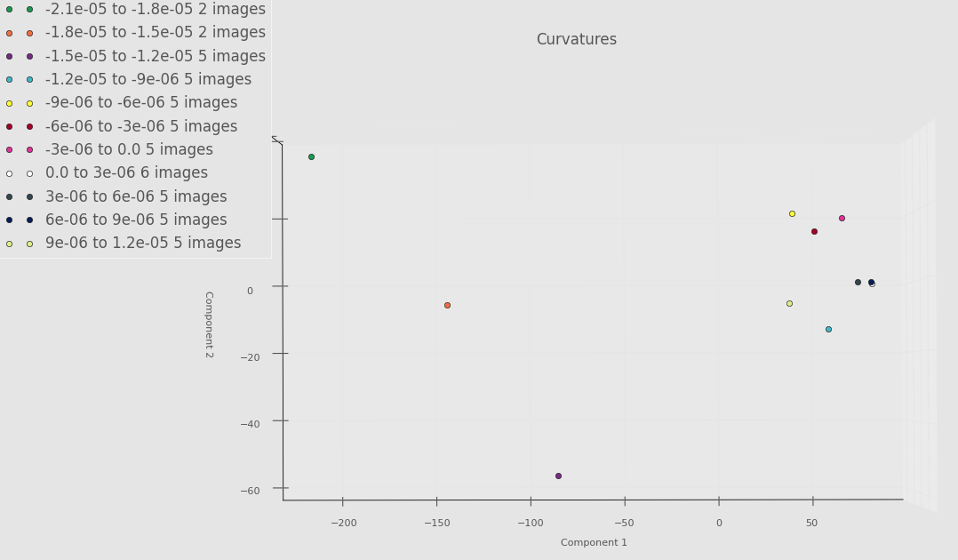
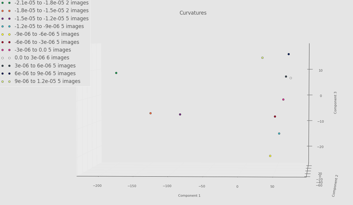
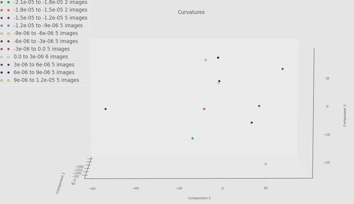
Example PCA
Below is an example PCA run on only a few images from each torus. Think of this as a proof of concept. Until we get everything ironed out, we don’t want to “waste priority” on PACE by constantly requesting lots of RAM. Even though there is something fishy going on with the Fourier basis, we still see some separation between some of the very negative Gaussian curvature bins and the rest of the bins. Whether or not this will persist once we’ve debugged everything remains to be seen.
Screenshot highlighting PCA component 1 versus PCA component 2 below.
Screenshot highlighting PCA component 1 versus PCA component 3 below.
Screenshot highlighting PCA component 2 versus PCA component 3 below.
Miscellaneous notes
We run the stats on PACE due to memory constraints. When we did a sample run with all of the data (using our flawed basis) to check that the runtime was reasonable, we found the output pickle file to be 62 GB (using 7 Fouier components and 7 Legendre components)! This raises the question of how many Fourier/Legendre components are necessary as we want to run on enough to capture trends, but we cannot just willy-nilly raise the number of components due to memory constaints. Advice on how to determine the optimal component number would be appreciated!
What do we wan out of this project?
As you may or may not recall, the workflow shown in update 3 is a little vauge once the “producde a model” step comes in. Now that we’re a little farther on and we’ve gone over the basics of Process-Structure models in class, we hope to clarify our end-of-class deliverable.
We want to use an ARMA-type process (because we suspect that we are only a weakly stationary process) to predict the evolution of the nematic director as a function of the local Gaussian curvature (process parameter 1) and the local Gaussian curvature gradient (process parameter 2). We would also like the model to be modular as we will later vary other process parameters (the activity, density of nematic, etc) and would like to be able to use this same framework. However, the additional experiments will happen after the class ends, so we will not worry about them for now.
Finally, more than just generating a model that works, we would like to be able to relate the model to the physics in this system.
How will we use November to get to our goal?
Before constructing the model, we need to make sure our PCA is correct. To do this we will: (1) Make sure that the data are being represented in the Fourier basis correctly. (2) We will figure out the optimal number of terms in the Fourier series and Legendre series we need to be able to properly represent our data. (3) Run statistics on the whole dataset (4) Determine how many components we need to keep in PCA using leave-one-out cross-validation (5) Develop an ARMA-type model (more on this as we learn more in class).