What is this post?

This will cover how I determine the number of componenets to use when representing my microstructure using a continuous basis function (rather than just the primative basis)

Our bases

We use both the Legendre polynomials (to represent the degree of alignment) and a Fourier series. The Legendre polynomial basis is already implremented in PyMKS. The Fourier basis is not yet integrated into the distributed PyMKS, but I have the most updated version (written by David) to use for my data. As a continuation from my last post, there was an error in the implementation of the Fourier basis, but it’s now been fixed. The data are discretized such that $\frac{1}{\Delta} \int_s m(h,x) dx = \sum_l m[l,s] \zeta_l (h)$ , where $m$ , $h$ , $s$ , and $x$ are the ususal variables to represent the microstate probability, the microstate itself, the discrete spatial bin, and the continuous spatial position, respectively. Here, $l$ represents the discrete local state, and $\zeta_l(h)$ is the appropriate orthogonal basis function. In this way we recast the original state space into the state space of the orthogonal function basis where each value of $l$ corresponds to a state in the new basis. For the degree of alignment we use the Legendre polynomials, $\zeta_l (h) = P_l (h) = \frac{1}{2^l l!} \frac{d^l}{dh^n} \left [ (h^2 -1)^l\right ]$ . For the orientation, we use a Fourier series, $\zeta_l (h) = \exp(i\frac{2 \pi l h}{P})$ , where P is the periodicity of the data. In our case, P is $\pi$ .

Note that for N states, the Legendre polynomials have $l$ range from $0$ to $N-1$ while for the Fourier series $l$ ranges from $-(N-1)/2$ to $(N-1)/2$ .

How many terms in the Fourier series do we need?

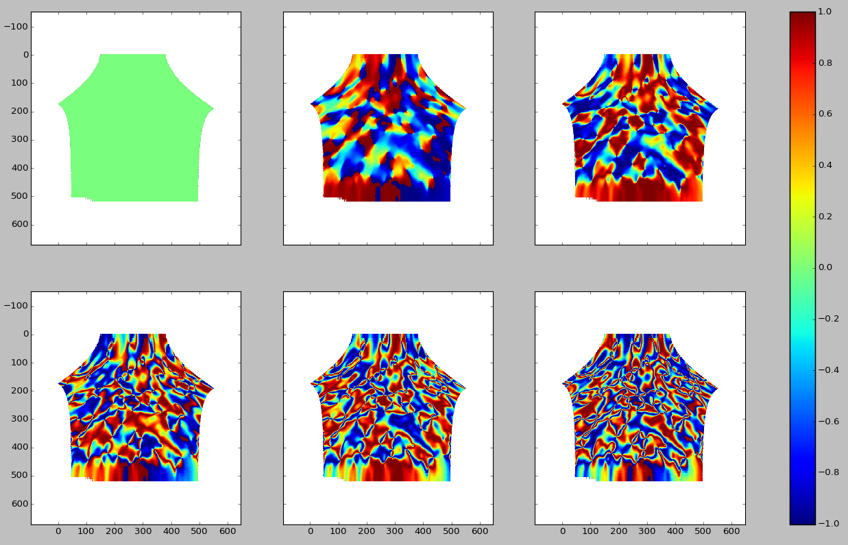
First, let’s take a look at the data in terms of the values for the different terms in the Fourier series. Starting in the upper left corner from from left to right we have the data as represented in the space of the 0th, 1st, 2nd, 2rd, 4th, and 5th positive Fourier component. Only ther real part is shown. The corresponding negative components have the same real part and so they are not shown. Note that the colorbar is accurate for all but the 0th component. That value is actually $1$ , not $0$ as the color would have you believe. I have checked this independently - it is a visual error due to the way I’m plotting and I haven’t changed it because I’m having some trouble getting matplotlib to do as I say.

Fourier basis 1

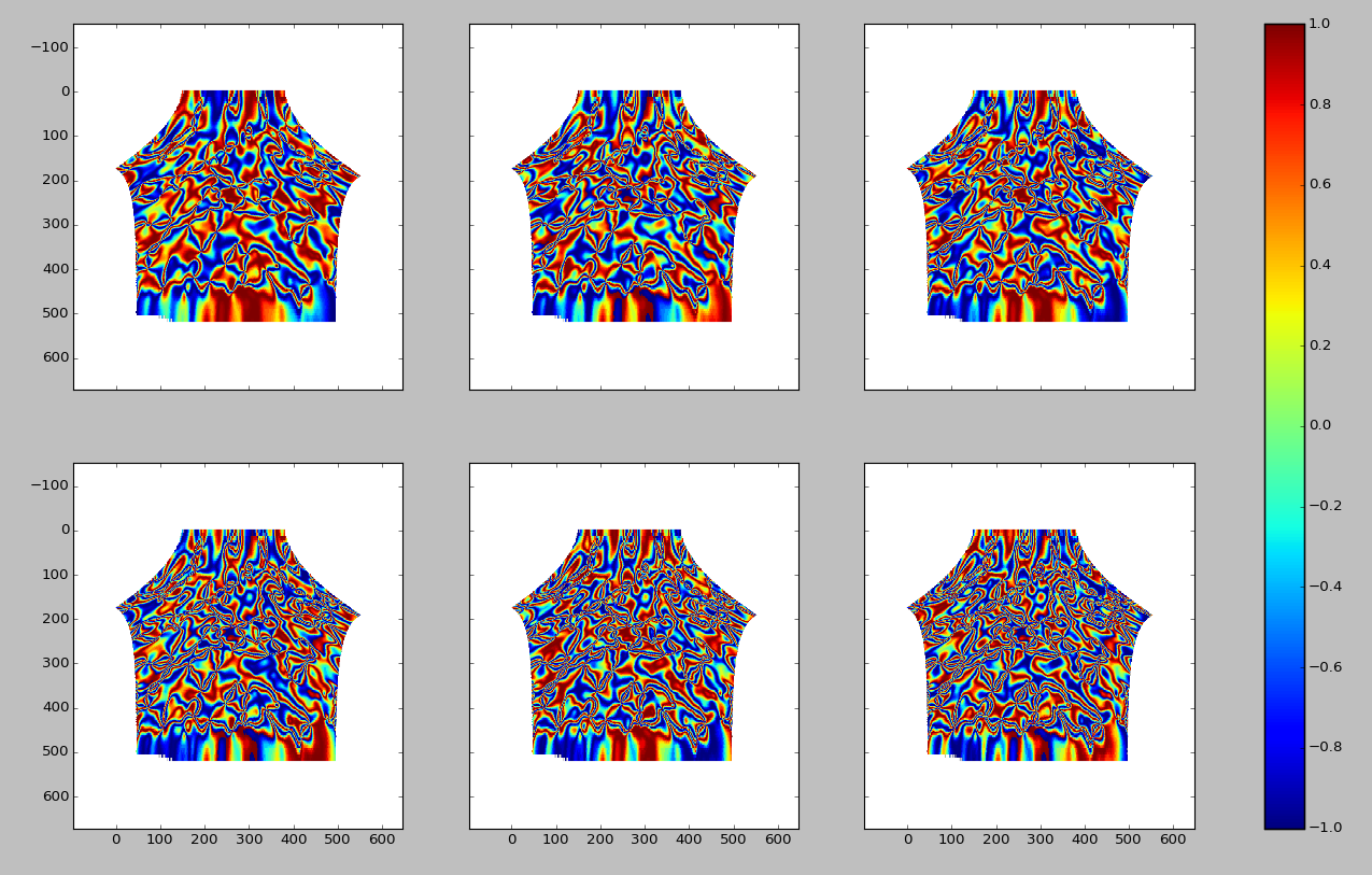
Physically, we interpret this space in terms of the spatial frequencies of the orientation data. This means that the 1st component is periodic on $[0,180]$ degrees, the 2nd component is periodic on $[0,90]$ degrees, the 4th component is periodic on $[0,45]$ degrees, etc. Simply by looking at the data it’s not obvious how many terms to keep. This also holds true when looking at even higher order terms. Below are the real parts of the 6th, 7th, 8th, 9th, 10th, and 11th positive Fourier components (again from left to right, starting at the upper left corner of the image).

Fourier basis 2

This can also be seen when looking at the average value and standard deviation for some Fourier terms for the example image.

State #	Fourier Term	Average	Standard Deviation
1	0	1.00	0.00
2	1	0.56	0.83
3	-1	0.56	0.83
4	2	0.18	0.98
5	-2	0.18	0.98
6	3	0.28	0.96
7	-3	0.28	0.96
8	4	0.10	1.00
9	-4	0.10	1.00
10	5	0.22	0.98
11	-5	0.22	0.98

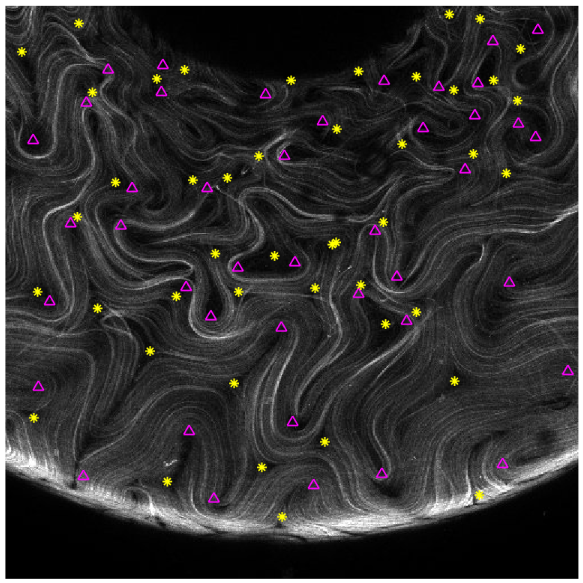
Apart from trying to reconstruct the original data from the fourier basis (which I’m not entirely certain how to do), we can also choose the number of states using the frequency arguement from earlier. From a sample image where the positive defects are pointed by the magenta triangles and the negative defects are pointed by the yellow asterisks, we can see that the spatial frequency needed to capture the spatial defect resolution would need a prohibitively high number of states. Here the defects serve as an structureal feature that we want to represent. As an example, if the distance between 2 defects is 1/10th of the image, we would need the $\pm 20^{th}$ Fourier term to fully capture this feature, corresponding to 41 terms in the Fourier series!

Defects

That makes a physical reason for the number of Fourier states not useful. This leaves us with a data-driven approach. What we’ll do is to run statistics and PCA on a subset of images using different numbers of terms. Then we can see the effect of the discretization of the final result and choose the number of states as the best comprimise between perfect representation and realistic computation time/resources. This will be detailed in a later post

How many Legendre terms do we need?

As with the Fourier series, let’s look at the data in the Legendre space. Starting from the upper left from from left to right we have the data as represented in the space of the 0th, 1st, 2nd, 2rd, 4th, and 5th Legendre polynomial.

Legendre basis 1

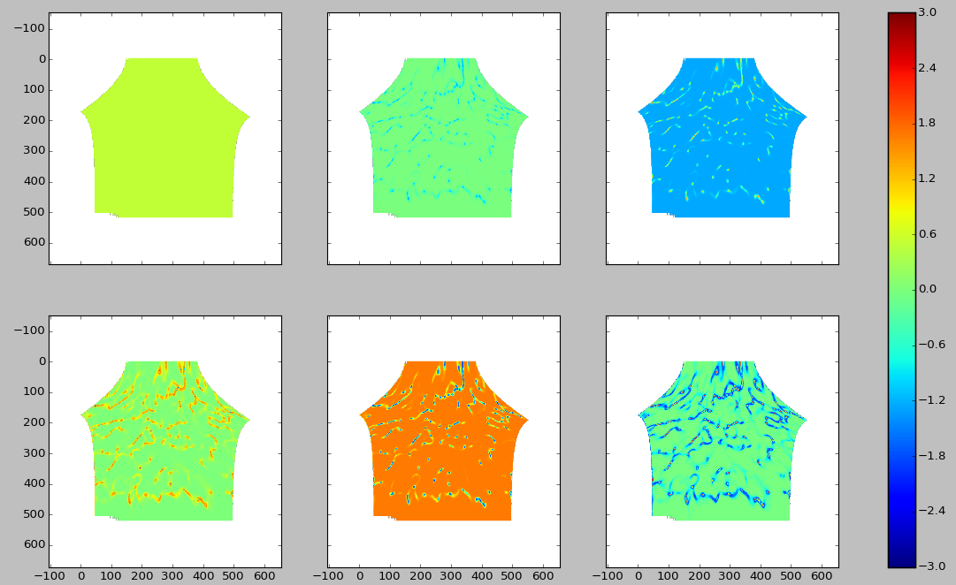
Here, the data are characterized by a small regions of values close to zero with the rest of the data with a value of 0.5 (out of a maximum of 1). This seems well-represented only taking the 0th and 1st term. To be safe, we will keep the 2nd term.

Thus, we need 3 states in the Legendre polynomials to represent the degree of alignment.