What is this post?

This will cover how I determine the number of componenets to use when representing part of my microstructure using the Fourier basis

Where are we with the Fourier basis?

Recall from last post that the data are discretized such that $\frac{1}{\Delta} \int_s m(h,x) dx = \sum_l m[l,s] \zeta_l (h)$ , where $m$ , $h$ , $s$ , and $x$ are the ususal variables to represent the microstate probability, the microstate itself, the discrete spatial bin, and the continuous spatial position, respectively. Here, $l$ represents the discrete local state, and $\zeta_l(h)$ is the appropriate orthogonal basis function. For the orientation, we use a Fourier series, $\zeta_l (h) = \exp(i\frac{2 \pi l h}{P})$ , where P is the periodicity of the data. In our case, P is $\pi$ .

Note that for N states, the Fourier series $l$ ranges from $-(N-1)/2$ to $(N-1)/2$ . Also from last time, recall that there was no obvious way to determine the optimal number of terms in the Fourier series; we finished with the conclusion that we would determine the number of terms in the Fourier series empirically. We will do this by computing stats/PCA on a small subset of images and looking at the captured variance for the first 10 components.

Limitations of this approach

Since we’re not running this on PACE, we’re limited to a very small subset of images (3 images for each of the 3 toroids … 9 images total). In addition, we can’t really look at more than 13 terms in the Fourier series. Anything else starts to run up against the amount of memory on the computer. While in principal we could get a better estimate of the optimal number of terms using more images, we should still be able to get an idea of how many terms we need. Basically, we’re relying on the fact that the most variance we have is going to come from the differences between the 3 toroids and not from the time-series images for a single toroid.

The captured variance

First we’re going to look at a plot of captured variance for the first 10 PCA components for different numbers of terms in the Fourier series.

Captured variance

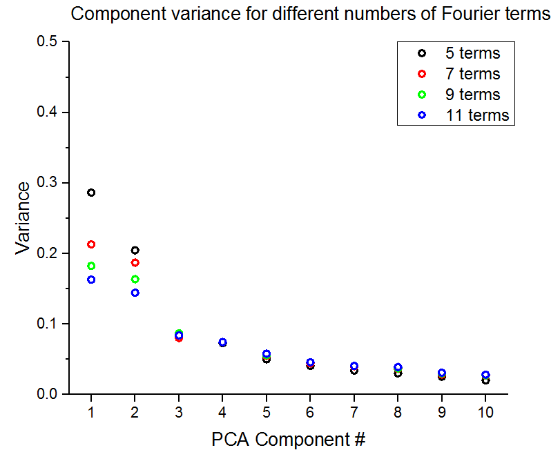
Right away we can see that no single component captures more than 30% of the variance, regardless of the number of terms used in the Fourier series. In face, note that the captured variance decreases as the number of terms in the Fourier series increases. Just to check, we can look as the cumulative variance captured in the table below as a function of the number of PCA components included for different numbers of terms in the Fourier series.

# Fourier Terms	PCA components
	2	4	6	8	10
5	0.491	0.648	0.739	0.803	0.859
7	0.400	0.555	0.654	0.731	0.789
9	0.346	0.508	0.610	0.688	0.745
11	0.307	0.465	0.569	0.649	0.705

It’s unfortunate that even with 10 componenets we are still capturing less than 90% of the variance. However, this does seem that there is no real reason to use more than 5 terms in the Fourier series. Just to confirm this, let’s look at some PCA plots.

PCA plots

Just as a starter, recall that these are only for 3 images for each torus, so we aren’t trying to say anything physical yet. All we’re doing is looking at the structure of the data transformed into PCA space to confirm that we don’t need to use more than 5 terms in the Fourier series.

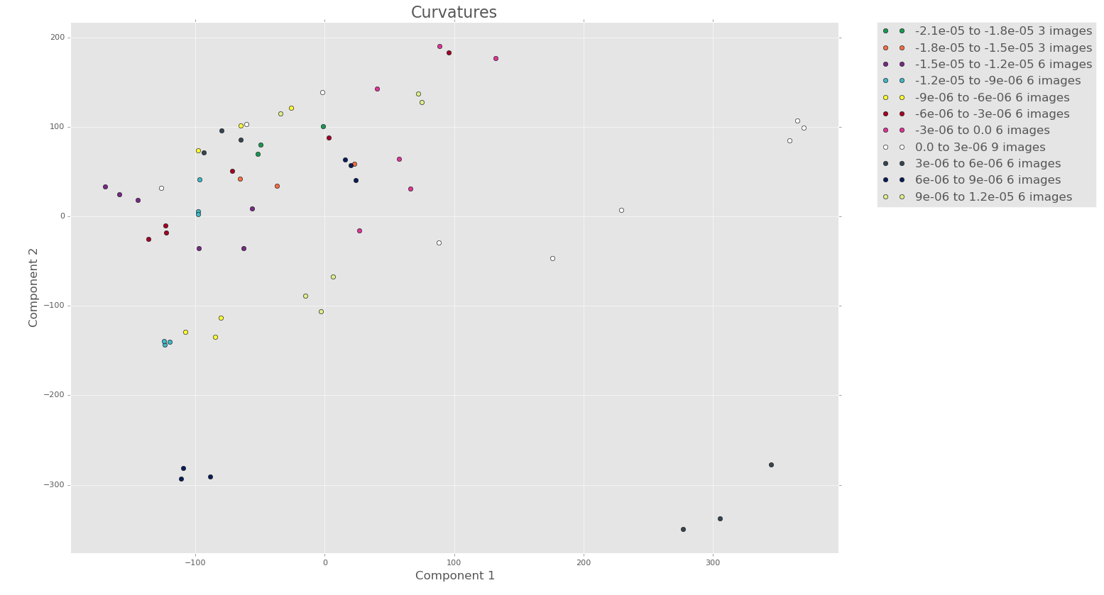
5 terms

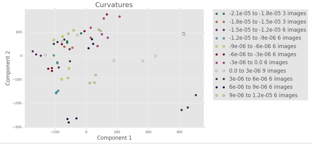
PCA 5 terms c1c2 PCA 5 terms c2c3 PCA 5 terms c1c3

There seems to be some good clustering, but we can’t say much until we look at the other PCA plots

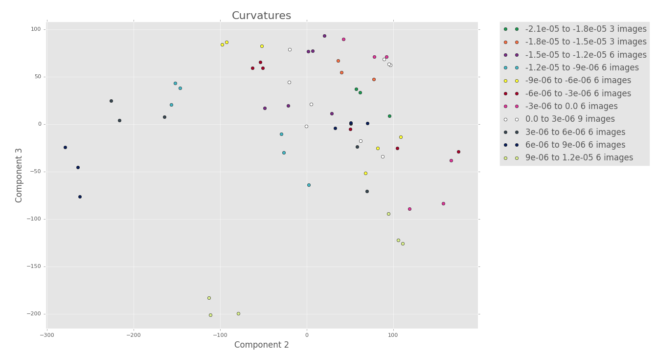
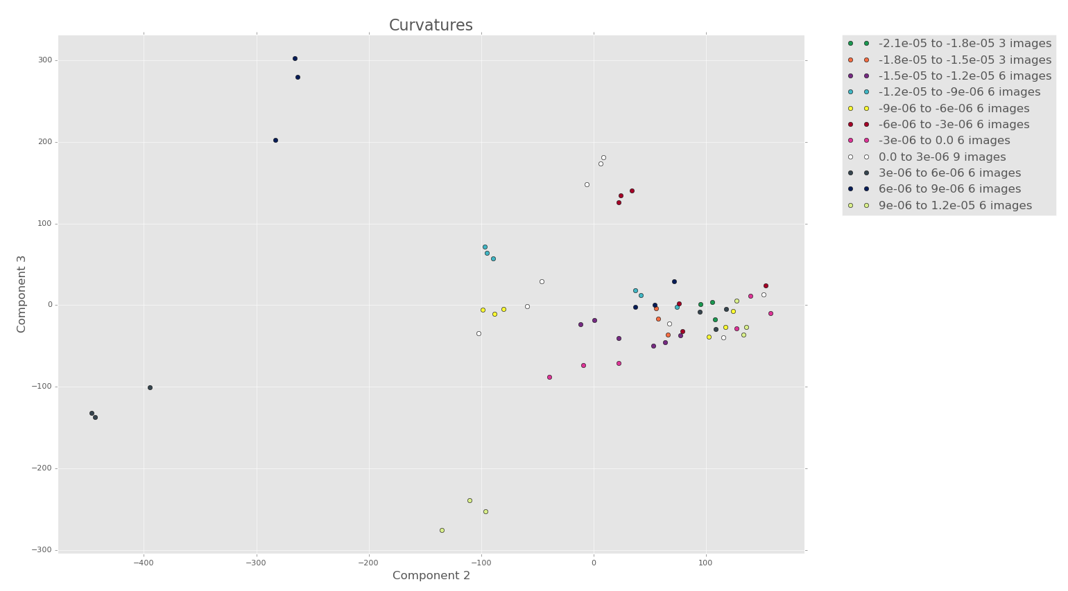
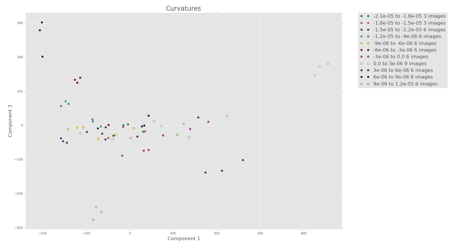
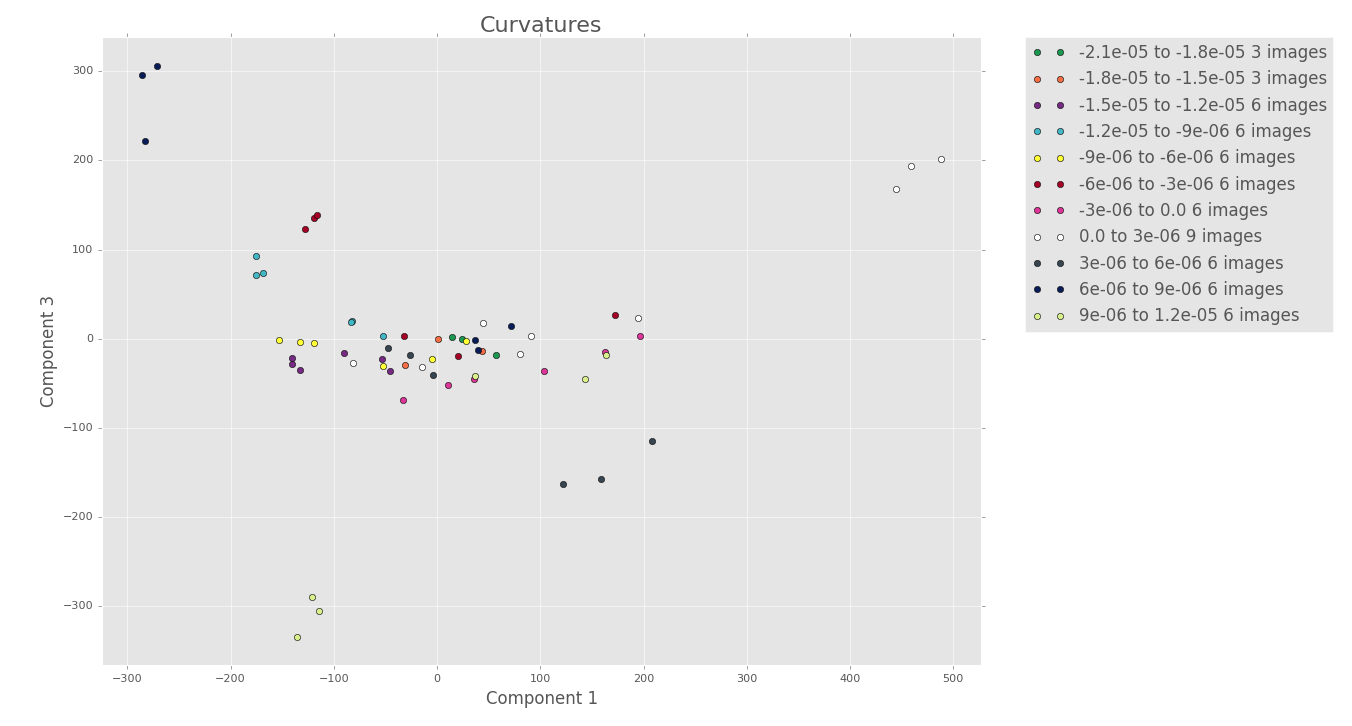
7 terms

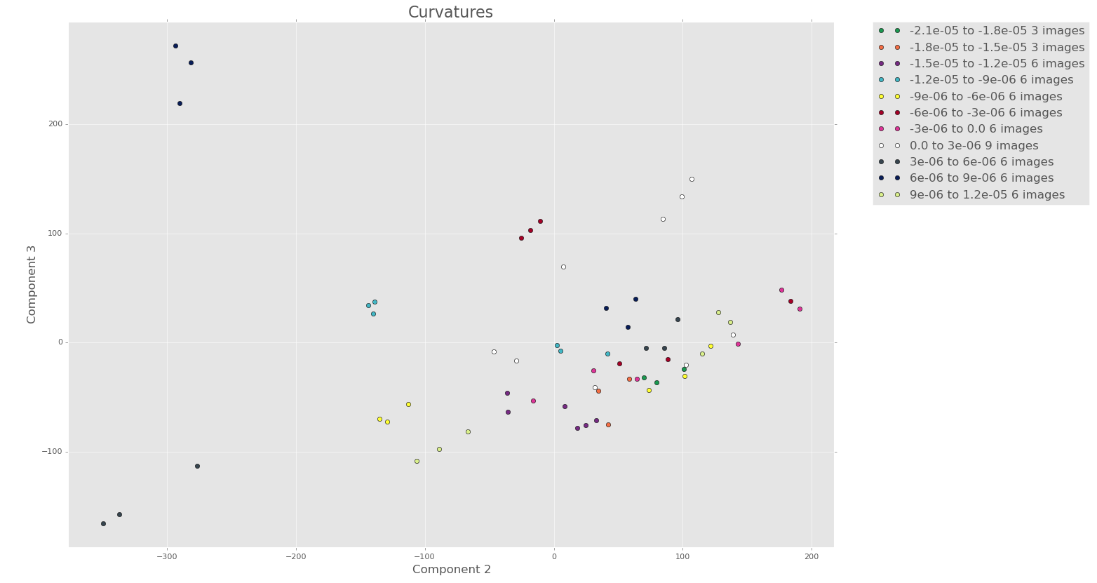
PCA 7 terms c1c2 PCA 7 terms c2c3 PCA 7 terms c1c3

Note how there seems to be more clustering/structure in the PCA plots of the first 3 components with 7 terms, even though less variance is captured!

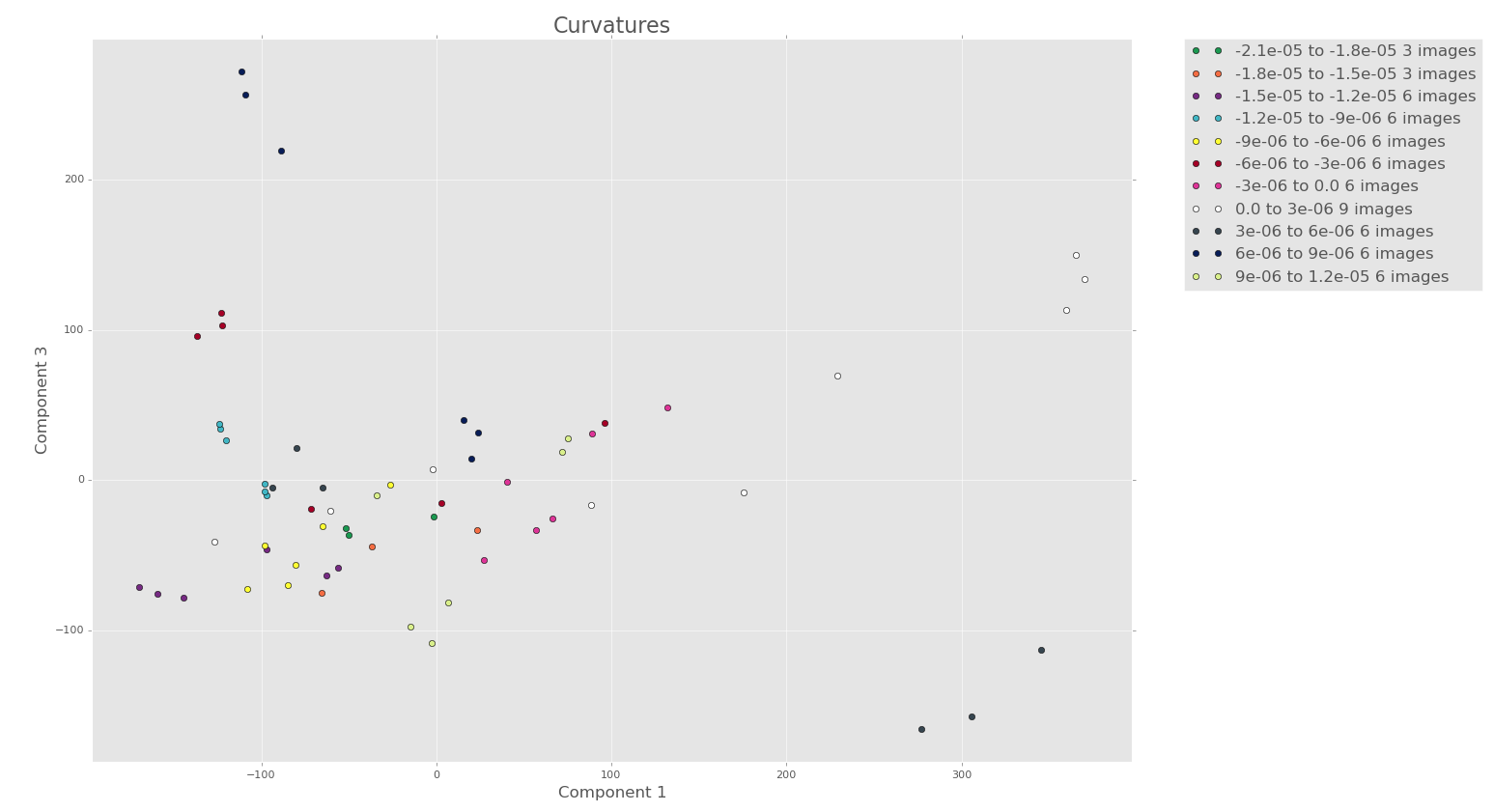
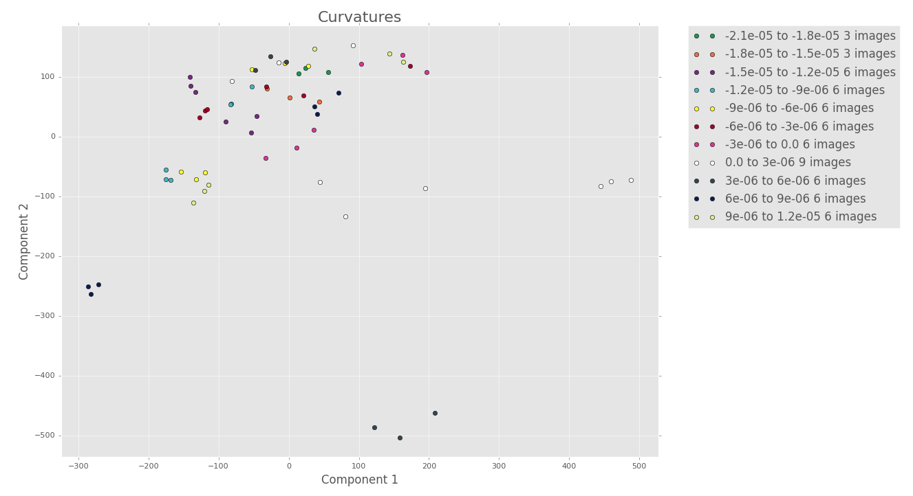
9 terms

PCA 9 terms c1c2 PCA 9 terms c2c3 PCA 9 terms c1c3

To the eye there doesn’t seem to be too much more structure when we look at the PCA for 9 terms.

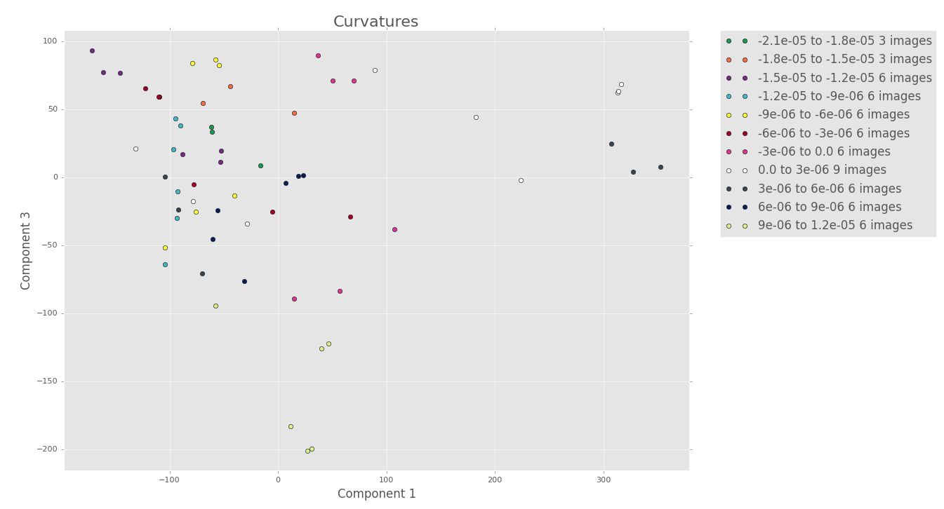
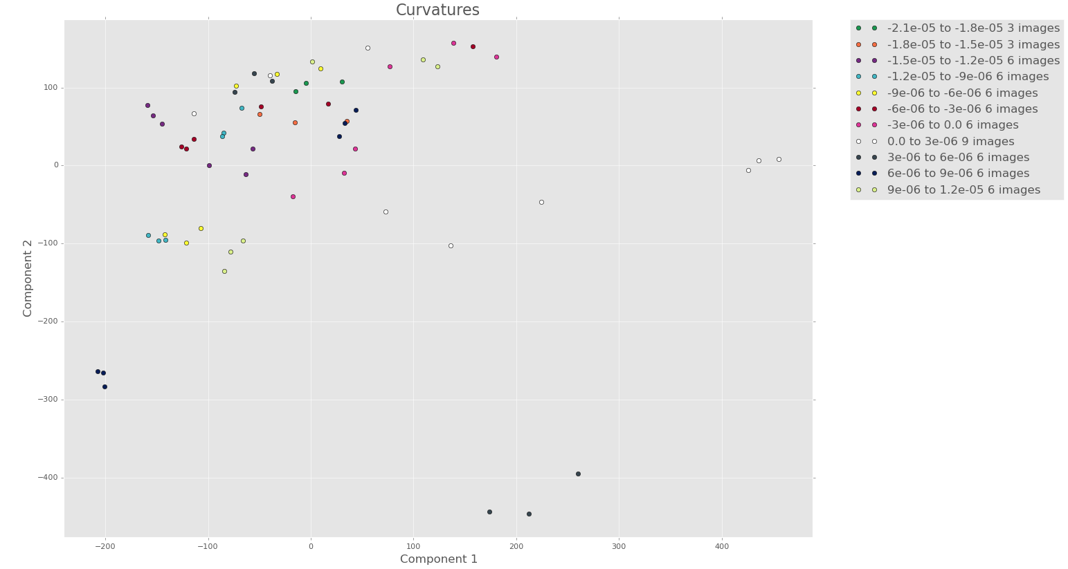
11 terms

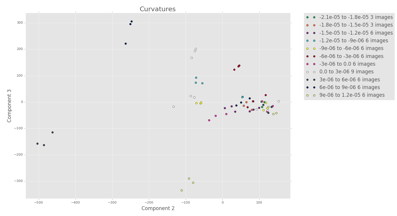
PCA 11 terms c1c2 PCA 11 terms c2c3 PCA 11 terms c1c3

When comparing the PCA plots for 7 terms with the ones for 11 terms above, there does seem to be more structure, but it’s hard to say. I don’t think that the added structure is worth the decreased variance and increased computation cost.

In conclusion…

We will use 7 Fourier terms as it seems to be the best balance of variance captured, structure/clustering in the PCA scores, and computation time/resources.