The sample images generated were very controlled. We were able to dictate the volume fraction of particles, the size of the particles, and even bias the distribution of the particle location to the top or bottom of the membrane. Even though we randomized the location of the particles, we still knew what to expect from analysis of the created files. This was very useful when comparing the results of the two-point statistics tool in MATlab to what we were expecting the results to be. This post talks about how our “fake” data analyzed using 2-point statistics and what the results tell us. The files representing data were created using the MATlab script “sample_creator.m” as described in the previous post. Four samples were created using different height ratios. The height ratio is the ratio of the thickness of the membrane to the distance between the slot-die and the substrate (height ratio = h/H). See Fig. 1 below for a refresher on these dimensions.
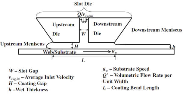 Fig. 1 – Slot-die extrusion membrane process diagram
Fig. 2 below shows the samples created by setting the height ratio to 0.25, 0.50, 0.75, and 1.00 respectively. Notice how the sample for h/H = 0.25 has a particle distribution that is more biased toward the bottom of the membrane, while the samples with h/H = 0.75 and h/H = 1.00 are biased toward the top. Also notice how there is no perceived bias for the h/H = 0.50 sample.
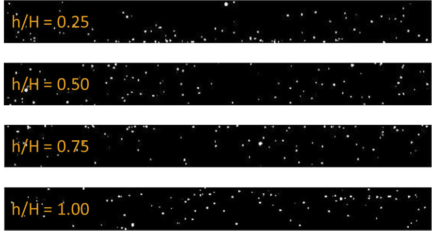 Fig. 2 – Generated samples with various height ratios
These samples were evaluated using two-point statistic MATlab code sound on the Material Informatics GitHub account. The function “PadState.m” creates a padding around the sample (as it is not recurring) and the function “CorrMaster.m” generates an auto-correlation. It is also easy to find the volume fraction as calculated by the auto-correlation using the CorrMaster function. This is valuable as the volume fraction gained from the two-point statistics was consistently within 5% of the volume fraction set in the creation of the samples. This helps to validate the accuracy of the CorrMaster function when used with our sample data to generate auto-correlations. The auto-correlations for each of the samples shown in Fig. 2 are shown below in Fig. 3.
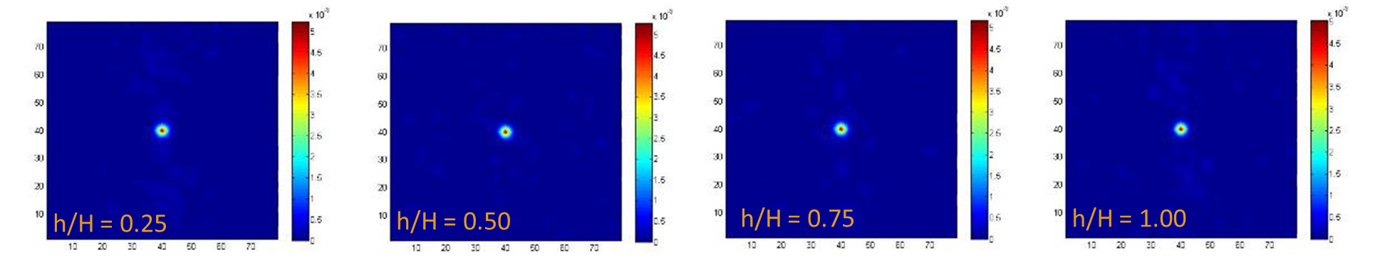 Fig. 3 – Auto-correlations of generated samples with varying height ratios
Notice that for the h/H = 0.50 sample, there is no noticeable pattern in the auto-correlation. For the other three, there is a higher probability of finding another particle above or below the first particle. This makes sense as the particles in the x-direction are made to be completely random, while the y-direction for these three samples are biased toward the top or bottom. Therefore, if there is one particle it is likely that another particle will be nearby in the y-direction. These findings are significant because we know that if we can get the data we receive from the CT scans to be in a form like the samples we have created, we will quickly be able to run 2-point statistics. This will hopefully go a long way in streamlining data analysis once we have data to analyze.