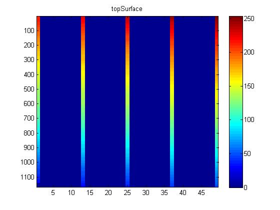
The next step in segementing the image data is using the edges that have been highlighted by hand for 5 of the image slices to crop the data. A MatLab script was created which would identify the colored upper and lower edges in each of the images. The figure below shows a sample contour plot of the top edge for a data set.
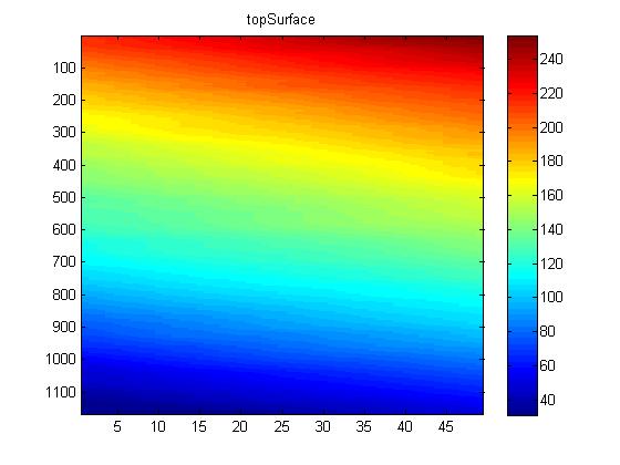
The edges for the image slices between the ones identified manually were found by linearly interpolating between the identified edges, as shown below. While there is some curvature in the membranes, this was found to be sufficiently accurate as there is already error due to the manual selection of the edges.
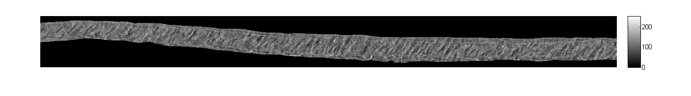
The data from the original CT data set could then be cropped using there upper and lower edges leaving just the composite membrane.
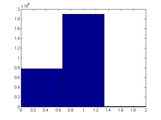
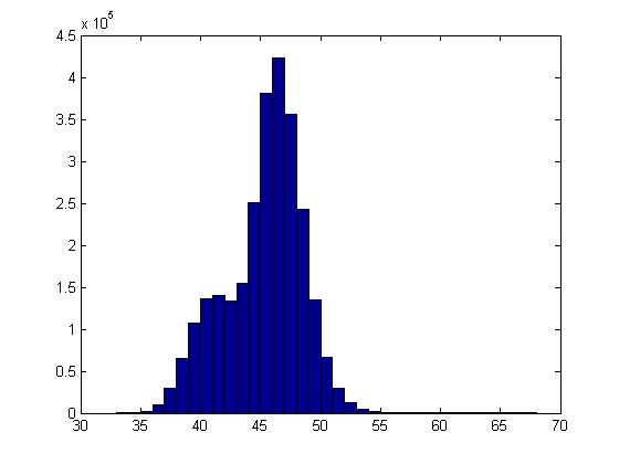
With finally having the membrane identified, the next step was to create a matrix with the pores, membrane, and particles identified. A histogram of the image intensities was created to help identify possible threshold limits. For the sharper, higher contrast images the drop in intensity for the pores could be identified easily. This is the shelf to the left of the large mid range bins as shown in the figure below.
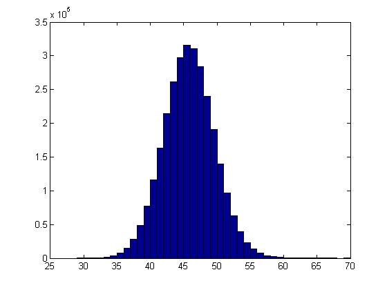
However, if the sharpness data set was low, the histogram took on a Gaussian shape and a limit for the pores could not easily be identified.
The threshold limit for the pores was manually changed until the pores were identified without selecting too much of the membrane material.
The limit for the particles was found by using the initial volume fraction of the glass particles in the solution of 0.005 so that the particle voxel fraction was close to this value.
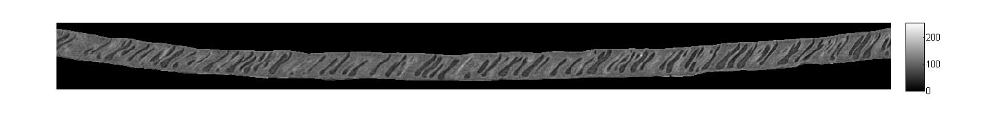
A sample final segmented image is shown below where 0 is a pore, 1 membrane, and 2 is a particle.