The purpose of this new blog post is to explain our followers how we proceeded to separate the output of our simulations into the 3 phases of interest for us.
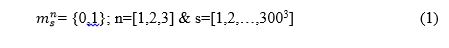
As explained in previous posts and in our presentation. We are using 300x300x300 microstructures and we have decided to break apart our microstructure into 3 different local states, the grain boundaries, the inside of the grains and the precipitates. We have also decided to assume that our microstructure is an Eigen-microstructure thus meaning that only one local state is possible to exist per spatial bin. Therefore our Microstructure Function looks like this:
The challenge that now our team faces is to be able to separate our data into the 3 local states defined by us. The output data that we obtain after performing the simulations in SPPARKS is a single row vector where each entry corresponds to a grain id, thus if a number is repeated this means that they correspond to a grain with the same orientation.
It is important to mention that we our initial available range of grain ids is from 1 to 1 million. After the simulation is performed some of this grain id’s disappear and other are repeated more often, since remember we are simulation grain growth. The following image is an example of the first couple of grain ids of an output of SPPARKS simulation.
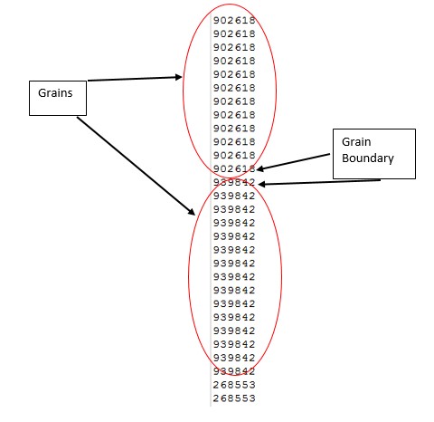
Now as the image states if a grain id is repeated right next to another one it means that those 2 grain ids correspond to the same grain and if they are different they correspond to a different grain. This is the first property that we are going to use in order to separate our grains from their boundaries.
The first thing we did was to reshape our data from a single row vector to a 300x300x300 matrix, since it is easier for us to operate with that.
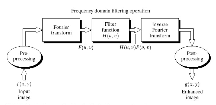
Now the question I am pretty sure all of you have is how are we going to look in every spatial and check if it belongs to the same grain and then assign it either a 0 or a 1 according to our microstructure function in a computationally efficient manner. Well we certainly did not used a “for” loop, we used the concept of filtering with FFTs (Fast Fourier Transform) explained by Dr. Kalidindi in class.
The key takeaways of this concept is that an image, or any data, can be filtered by taking advantage of the convolution property of FFTs. Theory states that a function in Fourier space when excited by an impulse function has an output spectrum equal to the convolution of the function and the input function. Thus if this impulse function is a filter of some sorts the result of this convolution is the filtered function through the defined filter. The following flowchart details this process clearly. Please refer to (resource 1, resource2 ) if more information about filtering with FFTs is desired.
Thus now our team needs to define a suitable filter for us to separate the grains from the grain boundaries. Thanks to the help of ( Ahmet Cecen and Yuksel Yabansu) our team was able to define the correct filter for our data.
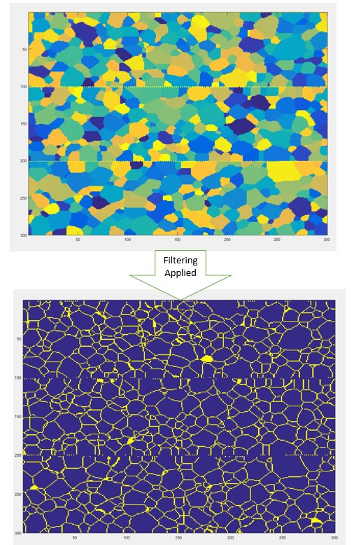
Remember how we mentioned that if a grain id was repeated it meant those two voxels belonged to the same grain, we expanded that into 3d. Thus we assigned a central voxel the value of -6 and each of its 6 neighbors, since it is in 3D, has a value of 1. Thus this means that if all the six neighbors have the same grain id as the value of the center voxel it means that all of them belong to the same grain, if not then the center voxel belongs to a grain boundary. Thus we used this filter, padded it with zeros to match the size of our microstructure and followed the flow chart above.
The results of this filtering is the following:
Finally we now just need to obtain the precipitates from our data. This step is significantly less complicates since SSPARKS by convention assigns the precipitate the biggest grain id. Thus we just needed to identify the location where the maximum grain ids were located and map them. Performing this last step on the previous images we obtain the image of the precipitate distribution, which is as follows:
As it can be observed this image corresponds to a uniform distribution of precipitates every determined voxels. It is important to mention that the precipitate distribution shown here is just an example for a test case. I hope this post was useful and please be on the lookout for new posts since we will be discussing the results of the 2 pt. statistics analysis performed on the simulations.