General Project Plan Recap
In class we defined four key steps describing particular stages of a material informatics project:
- Defining microstructure function
- Obtaining 2 point statistics
- Using PCA for dimensionality reduction
- Creating PSP linkage models
Our group has begun to extend our workflow forward and we now have some preliminary results for step 2: obtaining spatial statistical information.
A More Formal Microstructure Function
David recently posted some information about how we are pinning our initial microstructures and segmenting the data into a three phase material. For We have defined our phases as the following values:
- 0: inside the grains
- 1: grain boundary
- 2: pin
We have also tweaked our workflow a bit. We will be generating our data on PACE as we have already stated, but we will be implementing another loop that will take out dump files (raw data), segment the image data in the dump files, run 2 point statistics on each image for the correlation between the grain boundary and pins, and eventually perform PCA. These will be implemented all in Python on PACE to speed up the process.
So What About the 2 Point Statistics?
As mentioned earlier we have begun exploring spatial correlations in PyMKS. Consider the first example that is on the PyMKS homepage (note: this includes some packages that aren’t needed just for the example, but they are some packages that we have found useful performing data manipulations):
import numpy as np
import matplotlib.pyplot as plt
import matplotlib.image as img
import sys
from pymks.datasets import make_microstructure
from pymks.tools import draw_microstructures
from pymks import PrimitiveBasis
from pymks.stats import correlate
from pymks.tools import draw_correlations
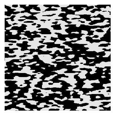
X_1 = make_microstructure(n_samples=1, size=(300,300))
draw_microstructures(X_1)
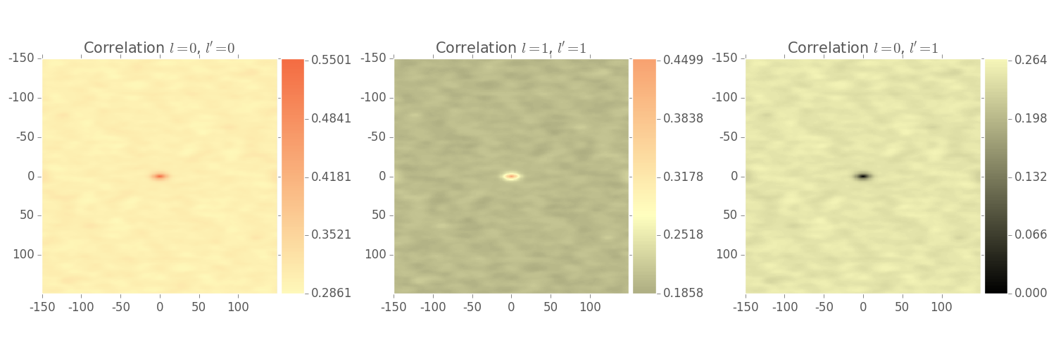
prim_basis = PrimitiveBasis(n_states=2, domain=[0,1])
X_ = prim_basis.discretize(X_1)
X_corr = correlate(X_, periodic_axes=[0,1])
print X_corr.shape
draw_correlations(X_corr[0])
This outputs a plot of our generated microstructure and the two point statistics of a 2 phase material seen below.
So we now have a better idea how 2 point statistics are implemented on a computer. But that’s just test data. We need to run this on our own data. We have a working Python script that can import images such as .png files as well as native Matlab .mat variables. But these aren’t worth showing quite yet, because our final plots need to take into account two things:
- Consider all three phases, and
- Perform the spatial correlation statistics in 3D.
Once these last two issues are addressed (which will be very soon) we will have another update exclusively on 2 point statistics related to our specific project. So stay tuned!