This is the post equivalent of the presentation given for our second progress report.

Outline

• Detailed Workflow and Data Pipeline
• Conditioning and Segmentation in Matlab (Step 1)
• 2 Point Statistics and PCA in Python (Steps 2, 3)
• Preliminary Results

Matlab

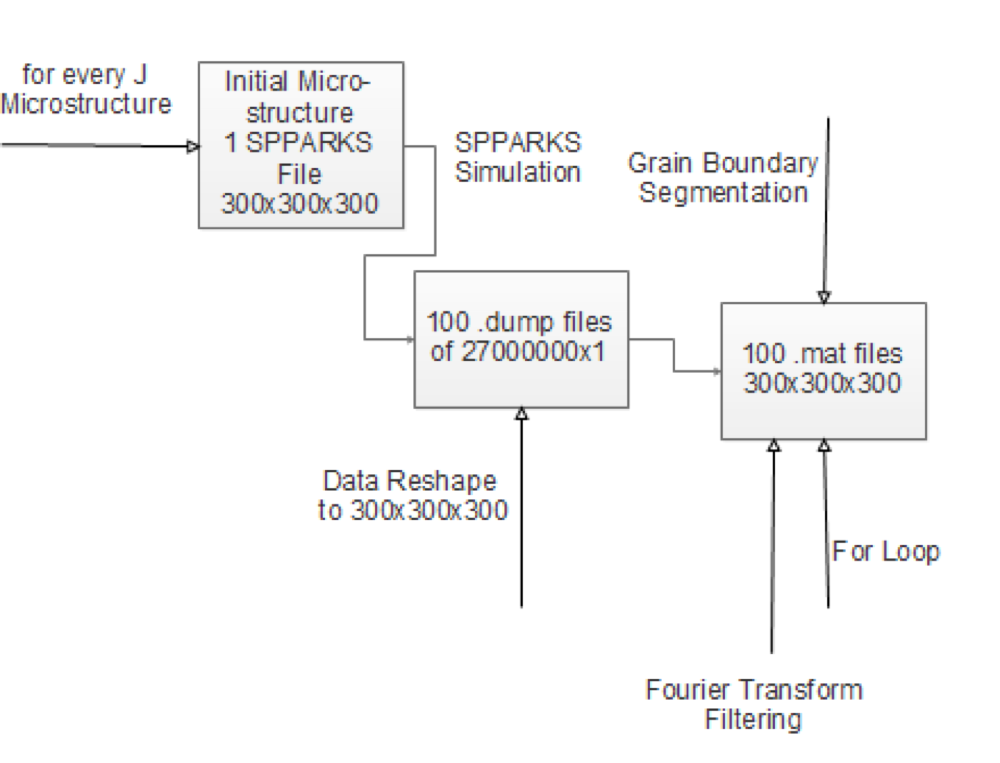
Image Segmentation

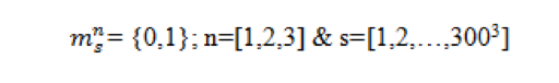
• Output from SPPARKS is a 27 million by one vector, reshape it to a 300X300X300 matrix.
• Each number corresponds to a grainID. Max value corresponds to a precipitate.
• We need to segment this data into our Microstructure Function.

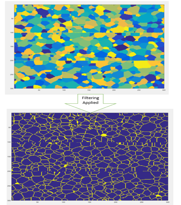
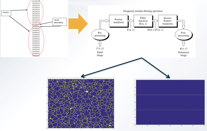
Obtaining Grain Boundary and Precipitates

Obtaining .mat files using PACE

• The issue is that the output from the filter are 3 images with 0 and 1.
• Which is desirable but we need it to change to one image with 3 distinct phases for us to input it to PyMKS.
• Made a for loop that will go through each .dumpfile and automatically segment it and save it as .mat file.

Python

Continuing where we left off in Matlab…

• Input: .mat files that only contain 0, 1, and 2 as values in an 300x300x300 array
  • Greatly reduces memory:
  • file.dump (~500MB) -> file.mat (~3MB)

2 Point Statistics Conditioning

• Initial size: (300, 300, 300) per file
• Loop that pulls each 100 outputs per simulation
  • Concatenates to feed directly into PyMKS
  • (n_samples, x, y, z) = (100, 300, 300, 300) per simulation

2 Point Statistics Computation

• 3 phase material -> 6 correlations
• Results in array of size (100, 300, 300, 300, 6)
  • Initially only care about one correlation: grain boundary and pins [1,2]
• After 2 point statistics computation: (100, 300, 300, 300, 1)

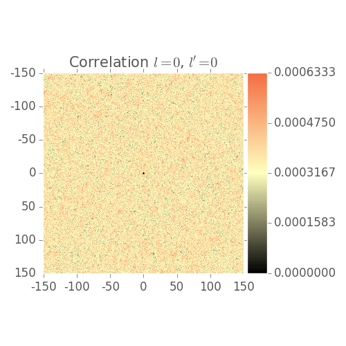
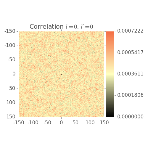
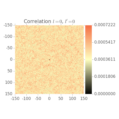
2 Point Statistics Plots

Shows 2 point statistics evolve over grain growth simulation

Note: Visualization issues:

1. Low volume fraction
2. Color bar not scaled correctly by default

PCA

• Forming the Data Matrix
  • Consider each 3D microstructure as long array
  • Reshape (100, 300, 300, 300) to (100, 300^3) = (100, 27,000,000)
• SciKit Learn Randomized PCA
  • Can specify number of PC values to output
  • Have tried: 2 and 3
    • Results in (100, 2) and (100, 3) matrix

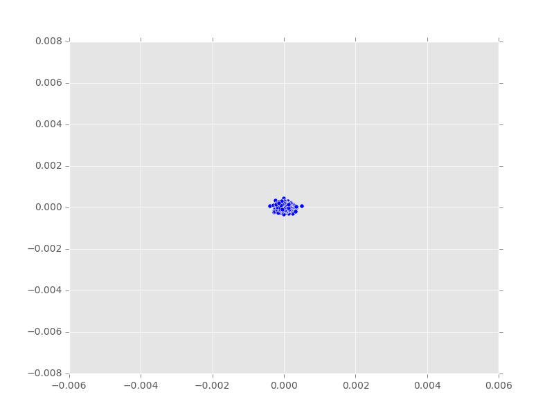
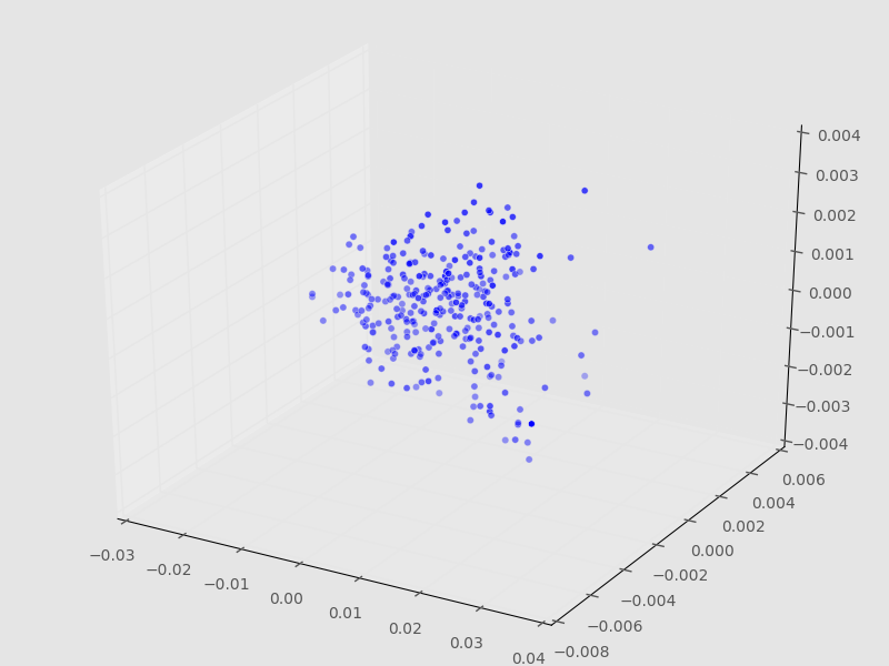
PCA Plots

• Final .mat files currently finishing on PACE
• Code pipeline is working but needs polishing
• Meaningless 2D and 3D example below

Next Steps

Bring analysis and visualization into 3D.

1. 2 point statistics of 3D data (longer computation)
2. Visualize 3D 2 point statistics results
3. Compute 3D PCA and Plot to see a path per simulation
4. Work with David Brough to use latest fitting code to create model

---

• ← Previous Post
• Next Post →