The purpose of this new blog post is to explain our followers how the desired property is obtained from the simulations performed. As our followers know we want to correlate grain growth to an initial distribution of insoluble precipitates. Thus since we are intending to obtain an effective property from our datasets we are facing a homogenization problem. As explained in previous posts. We are using 300x300x300 microstructures and we and we are using Kinetic Monte-Carlo model to simulate this “pinned” grain growth. Also in previous post we mentioned that we were able to extract our microstructure function from the simulation results.
At this point we have successfully ran 100 simulations each one of them with a different initial distribution of precipitates. Each simulation outputs 100 different snapshots that also will allow us to observe an evolution of how the grain grows. Nevertheless we still need to define a way to extract the grain size distribution from our data. In previous post we mentioned that we were able to obtain a .mat file that contains information about the grain, the grain boundary and the precipitate. This .mat file consists of a 300x300x300 matrix in which the inside of the grain is represented by a 0, the grain boundary by a 1 and the precipitate by a 2.
Thus we somehow need to use this file to obtain information about the grain size distribution at the end of the SPPARKS simulation. We exposed this situation to Dr. Kalidindi and he wisely suggested us to use chord-length distribution. The way chord length distribution is obtained is shown in the following figure.
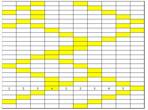
As it can be observed from the figure chord-length distribution consists on placing various cords of different sizes along one direction and counting the frequency of them, rendering a plot similar to a histogram. The most direct way is to use the 3 orthogonal directions, since a line in any different direction will bring up more issues since now you need to define how to obtain that line and also the grains will not finish at a pixel thus we decided to only use the 3 orthogonal directions. Also it is important to mention that since we have periodic boundaries the chords can wrap around for those grains located in the edge of the microstructure.
The way we implemented this algorithm was the following:
-
Obtain the chord length distribution along the x direction of the 300x300x300 Microstructure. This results in a 1x300 vector containing the frequency that each chord, from the size of 1 to 300, occurs in that direction.
-
Obtain the chord length distribution along the y direction of the 300x300x300 Microstructure. This results in a 1x300 vector containing the frequency that each chord, from the size of 1 to 300, occurs in that direction.
-
Obtain the chord length distribution along the z direction of the 300x300x300 Microstructure. This results in a 1x300 vector containing the frequency that each chord, from the size of 1 to 300, occurs in that direction.
-
Take the average of this 3 different vector and obtain a 1x300 vector with the average frequency of chord lengths in all directions.
The result is a histogram and an image of it looks like the following.
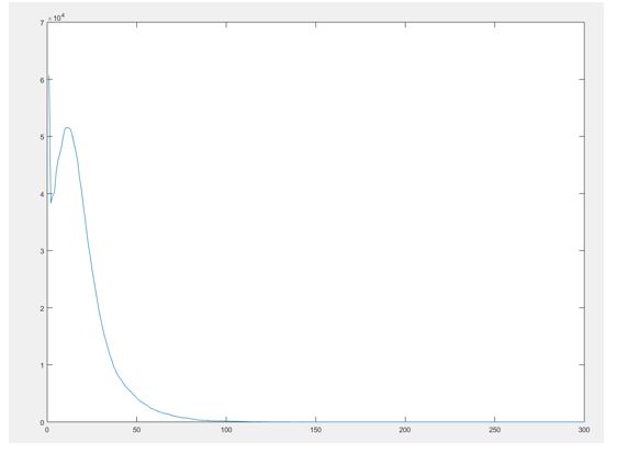
It can be noticed that a sharp peak of chords of length 1 exists. After further looking into this issue it was noted that the algorithm we used to segment our data, detailed in a previous post, causes come of the boundaries to be either extended or blurred, causing an increase in the chord of length one, this effect can be clearly observed in the following figure.
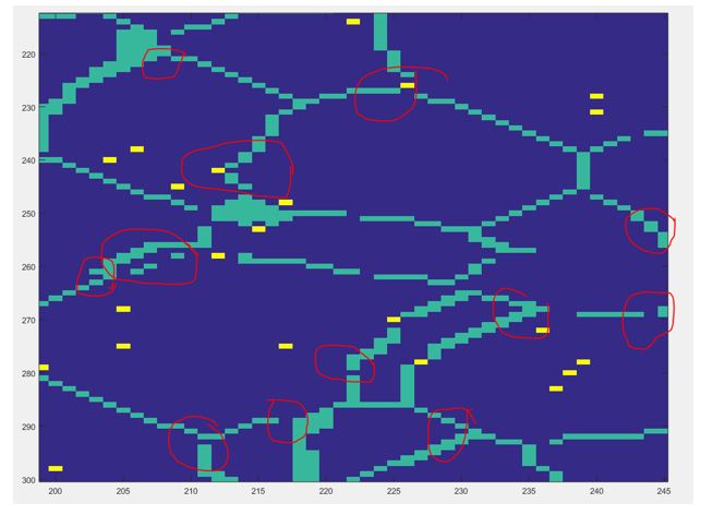
Therefore we need to find a way to address this issue since it might affect further analysis of the data like PCA since we know it is extremely data sensitive. Please be on the lookout for the next posts since we will detail how this chord-length distribution will be used to in the PCA analysis.