Typical Reconstruction problem
In a typical reconstruction problem the formulation showed below is used to reconstruct the microstructure.
The terms $|M_k^p|$ and $|M_k^n|$ are found from the autocorrelations of the discritized phases while $F_k^{pn}$ is the cross correlation. Typically the microstructure is reconstructed using a guess for the phase information pertaining to $e_k^i\theta$. However this reconstruction method is not applicable to our problem since we do not have a full set of statistics, nor the cross correlation. We are missing crucial datum to help us get the phase data which is one of the main reasons that the answer to the problem is non unique.
Database approach
Our new approach to this problem will be to explore if we can make a match using PCA as an objective means of comparing the scattering images and a handful of simulated microstructures. In order to do this we want to look at the microstructures in PCA space and see if clustering still occurs with the missing beam stop. We have decided to do PCA on the fourier representations of the autocorrelations of the simulated microstructures. This is logical since the conversion to real space would just present more work than necessary. We have done PCA on 180 simulated microstructures for now to observe preliminary results (we have plenty more to do). For these 180 microstructures we have decided to control the volume fraction, the average spacing between particles, as well as the size of the particles. The shape of these particles in this case is rectangular. The PCA of the untouched microstructures are first shown. A beamstop correction is than applied to the simulated microstructures, and PCA is performed once again.
PCA1: Untouched Microstructures
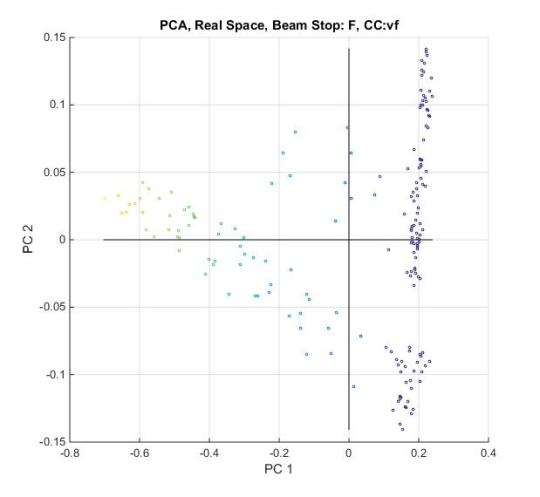
As a sanity check we will look at the PCA of the microstructures from the real space (i.e. equivalent 2-pt statistics) and compare to the PCA of the autocorrrelation in fourier space. The PCA observations are color coded according to volume fraction right now. The darker the color the higher the crystallinity. volume fraction
Real PCA
Fourier PCA
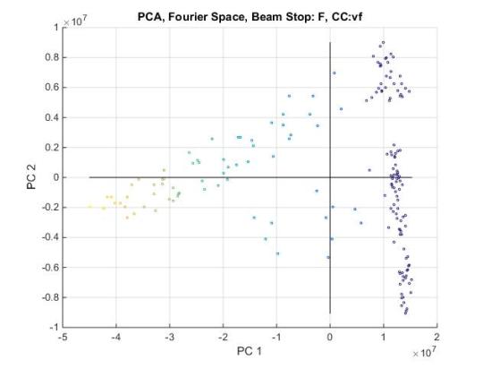
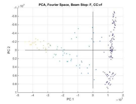
If we flip this PCA and compare to the real pca we can see the clustering patterns appear identical
Flip Fourier PCA
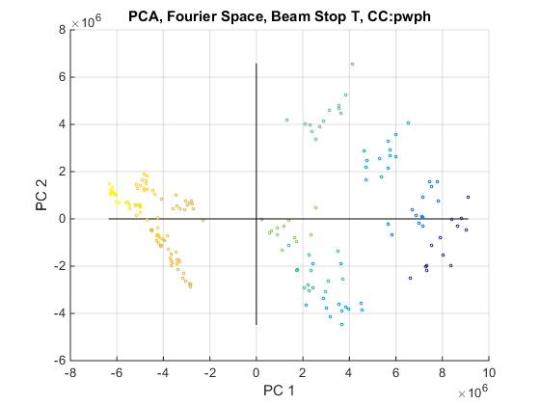
PCA2: Beam Stop applied to Microstructures
Now if we added the beam stop (took out data from center points) and performed PCA we get the following results.
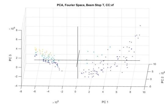
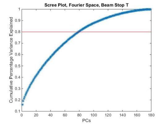
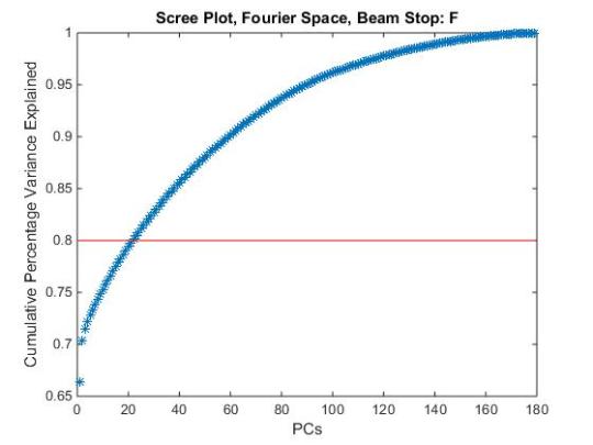
We can see that the observations appear to still appear to cluster somewhat according to volume fraction. We should also compare the scree plots between the untouched PCA and the PCA with the beamstop applied.
Take a look at the scree plots
Now we want to look at how much variance is captured by the principle components using scree plots. Observing the scree plots we see that it takes many more principle components to describe 80% of the variance when the beamstop is applied to the image. 80% is arbitrarily chosen. However just observeing the first 3 PCs on the scree plot shows that up to ~73% of the variance is accounted for when the beam stop is not included. This is in contrast to only ~23% of the variance accounted for within the first three PCs when the beam stop is included. This implies information within the beamstop contains a high amount of variance between microstructures
We ultiamtely want to see if we have any other clustering due to the parameters that we directly control. Performing the PCA and color coding according to spacing also does not give a definitive result. However, if we color code the pca according to “particle” size, we can start to observe clustering. In this case the darker the color the larger the particle. In these trials of PCA the particles all have the same shape.
PCA2: “Particle” Size Color Coded
NOTE: This Post was edited 11/23 to reflect new results