What are we looking at again?
This post will approach how the intesity images are seen in a more intuitive way. This post will try to draw parrallels to more familiar concepts in order to draw parrallels to what we have, what we do not have, and what in the end makes reconstruction such a difficult task in our case.
Start off with something familiar.
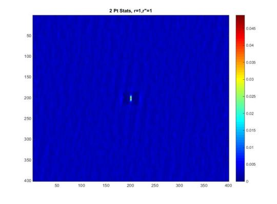
Let us start out with a simple simulated microstructure. Let us characterize the black shapes as the crystalline phase and white as the amorphous phase. If we were to find the autocorrelation/2-pt statistics of this specific microstructure it would look like the below image.
Simulated microstructure
2-pt stats
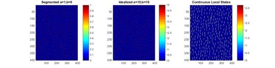
Compare the different possibilities of local states
The 2-pt statistics is from the microstructure discritized with 0s and 1s, this results in only the selected phase equal to 1 contributing to the autocorrelation. This 2-pt statistics shows our material system is 5% crystalline. However our material system of the real microstructure could be characterized as continuous local states, or we could idealize the two phase system and assume two discrete values for each phase(could be [69,78]…[200,300]…[3,5]…etc). Being not discritized into 0s and 1s complicate matters as the autocorrelation divided by the space no longer simply gives us the familiar 2-pt statistics. If we observe the resulting contours of a scaled image the contours of the idealized and segmented systems appear comparable while the contours of the continuous state microstructure may not be directly comparable. If we could assume the idealized system The most obvious approach would be to find a way to convert an autocorrelation of 2 given numbers to an equivalent autocorrelation of an image comprising of 0s, and 1s. However, we do not know how to make this conversion, or if it is possible.
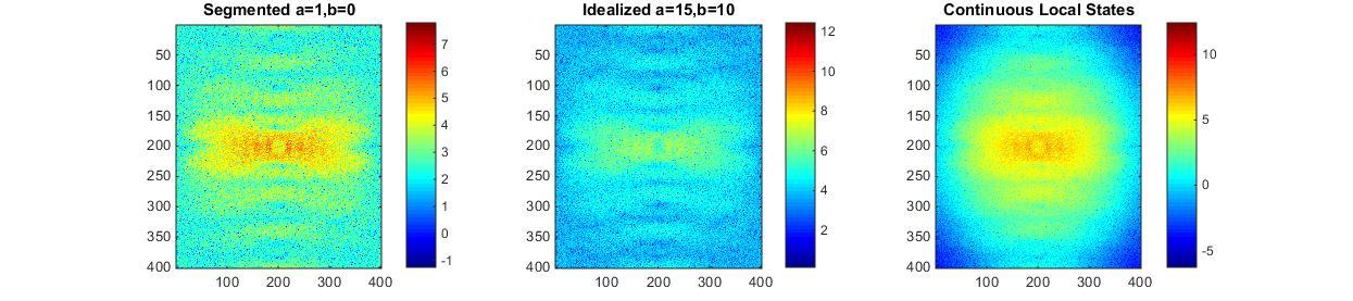
Mirostructures
Autocorrelation of Segmented Image, Idealized 2-Phase, Continuous Phase
But thats not what we have!
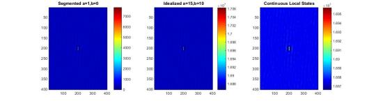
However, the scattered images are in fourier spaces so lets take a step back. We will find the autocorrelation in fourier space of all of the images above.
Autocorrelations in Fourier Space
Approaching the problem as an idealized 2-phase system
If we approached the problem as an idealized 2-phase system we could use the equations below to discern the value given to the phases which would give us criteria to apply when approaching the reconstruction of the microstructure. Using known properties of the autocorrelation we could determine the mean of the electron density. From domain knowledge we also know we can find the difference of electron density. This would be great but this is where our problems just start.
That beam stop again????
Now in order to have a true representation of the data that we have, we have to pluck out the values at the center of the autocorrelation in fourier space. This destroys the relationship we had previously defined. We also do not know if the idealization assumption is applicable given the difference from the scatter plots shown above. Our scatter plot of the idealized system would look like something below.
Scatter Simulation

Why can’t we just fit data there?
We previously came up with the idea to fit the data at the beam stop with a gaussian. This approach may have been unduly. The justification behind the fit was that a gaussian in real space is still a gaussian when converted into fourier space. This allows the shape of 2-pt statistics to be somewhat preserved knowing the shape of 2-pt statistics from experience starts off high and trails off to smaller values away from the center value. However, knowing that the fourier transform creates orthonormal basis the information at the beam stop is independent of the rest of the information. Knowing this inforamtion, the use of a gaussian as an approximation may be ill advised.
Exploring a database approach
Knowing this information we have decided to approach the problem with a database approach. This involves simulating a large amount of microstructure and trying to match the autocorrelation using certain thresholds. These thresholds will be based on shape. Going through this process has been useful as we see that it may be necessary to model the system with continuous states rather than idealized given how different the scattering patterns appear.