Process-Structure Linkages in Simulated LENS-type Additive Manufacturing Microstructures
Introduction
The LENS additive manufacturing process creates fully-dense alloy components with process-dependent microstructure. In this project we investigate the morphology of the microstructure crystal grains and it’s dependence on process parameters using a data science approach. A simulated dataset shared with us through Harvard’s Dataverse was subjected to a data science approach. The dataset’s creator Theron Rogers of Sandia National Labs has been our collaborator and domain expert, guiding the direction of the project. More detail can be found here.
Motivation
The LENS deposit physical properties are governed by the microstructure which is a function of the process parameters. We would like to be able to design the function and physical properties of the LENS-made components by using Process-Structure-Property Linkages. The focus of this project is to create Process-Structure Linkages.
Objective
The objective of this project was to extract Process-Structure Linkages from the simulated dataset. The grain size- and shape-distribution was specified as an important structure metric. The general direction of the project became extraction of grain patterns with respect to simulation process parameters. The linkages map a parameter combination to a unique microstructure in PC-space.
Approach and Workflow
The dataset represents 1799 unique 3D digital microstructures created by SPPARKS monte carlo simulations. Each structure occupies a 300x300x200 unit volume and is associated with a unique set of processing parameters listed below:
- (X/XY)Scan Pattern Linear and layer-by-layer cross-hatch
- (W)Melt spot width
- (V)Velocity
- (D)Melt spot depth
- (L)Melt spot tail length
- (HAZ)Heat-affected-zone width
- (T)Heat-affected-zone tail length
The 1799 unique microstructures have a variety of grain size and shape distributions, and example of which is shown below. The pseudo-periodic nature present in all these structures owes itself to the linear-serpentine scan pattern of the heat source in the simulation which mimics the movement of the LENS deposition nozzle and deposit formation.
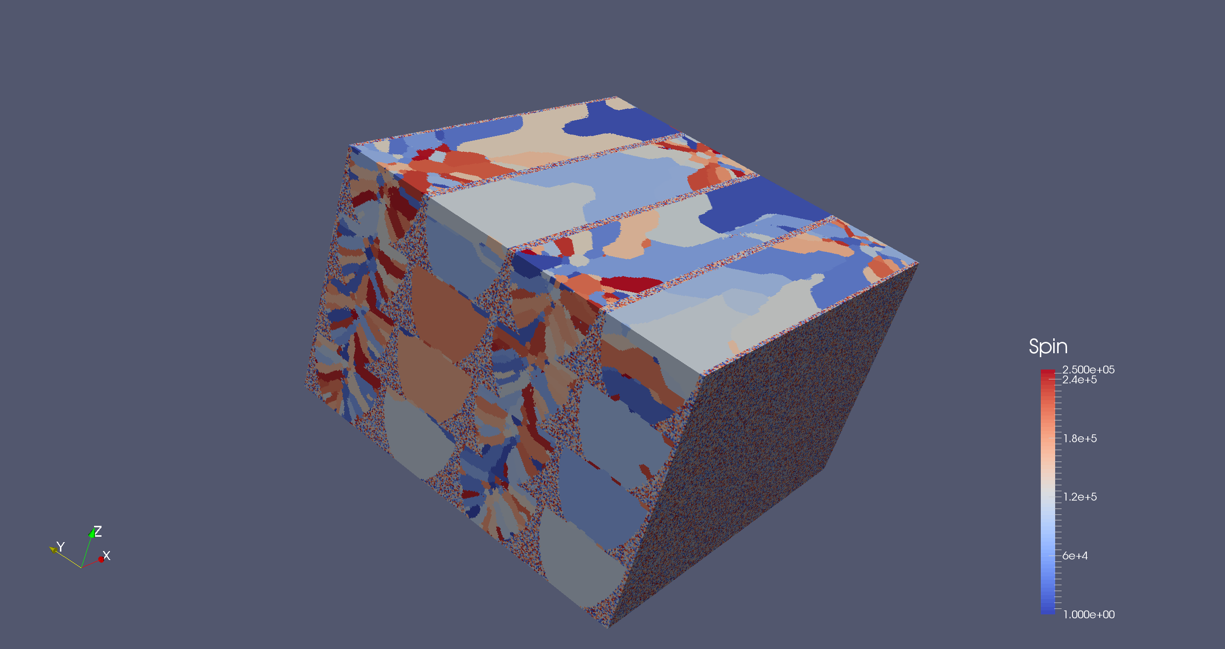 Fig.1. Example microstructure with parameter combination: T=20, X, V=2.5, W=60, D=100, L=50, HAZ=5
As received, the data in the dataset was organized in a folder tree, each branch of which defined a microstructure with a unique parameter combination. A code was written to navigate these branches, access the microstructure, and collect metadata (the process parameter combinations). A detailed explanation here.
The journey to extract the Process-Structure linkage is summarized in the worklfow diagram below:
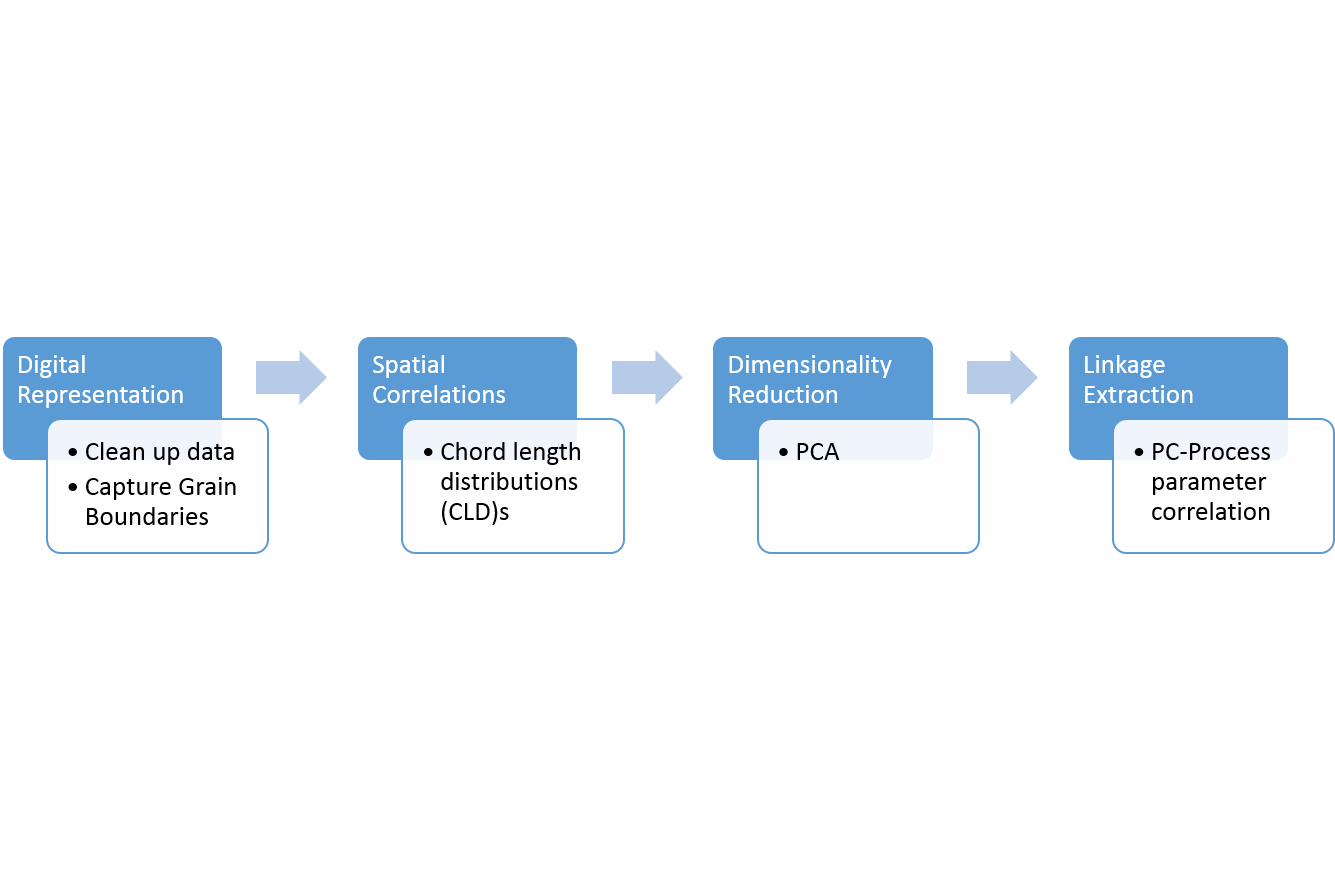 Fig.2. Workflow
In the Digital Representation step the data is processed and transformed into a computationally-convenient form, after which the microstructure is subjected to grain-boundary segmentation. The Spatial Correlations within the microstructure can be interpreted in different ways but we selected 2-point statistics and Chord-Length-Distributions (CLD) in this step. Details here and here and here. Both 2pt-statistics and CLDs are different statistical descriptions of microstructure. The 1799 microstructures are interpreted with a set of 1799 2-pt statistics and a set of 1799 CLDs. Before a linkage is built, the variance in each set is quantified and reduced in dimensionality using Principal Component Analysis (PCA). The PC space is truncated to a handful of PCs immensely reducing complexity yet capturing most of the variance.
The Process-Structure linkages are formulated to answer either of two questions:
- Given the process parameters what microstructure do they create? (Forward linkage)
- Given a microstructure, what Process parameters are needed to create it? (Inverse linkage)
The linkages are extracted by using linear polynomial regression.
Results
The CLD statistics were more appropriate to the structure information we wished to quantify. The results of PCA on CLD sets of the entire dataset are presented below.
Data Visualization in PC Space
The 1799 structures are plotted below in PC space, along with an accumulated variance plot.
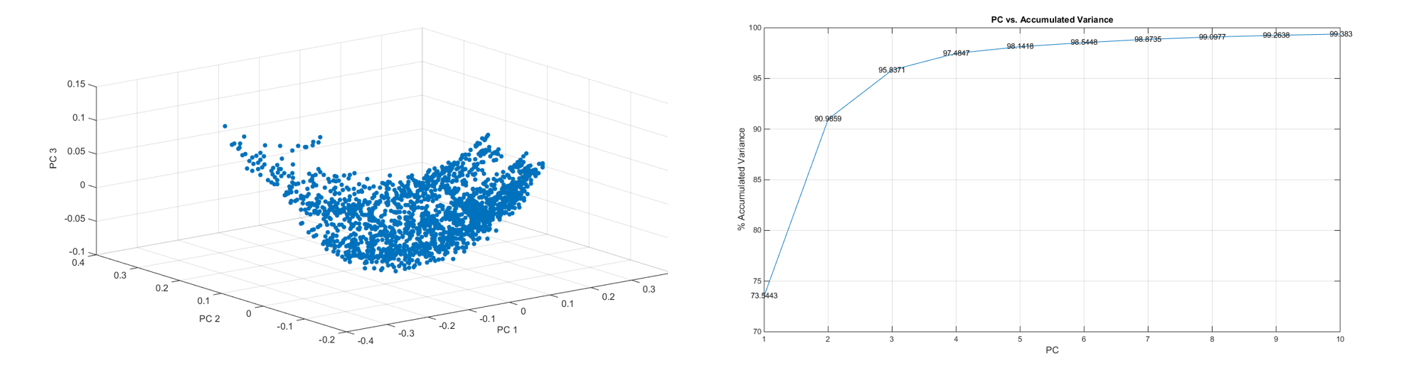 Fig.3. The CLD variance in PC space and corresponding accumulated variance plot
The separation of structures with respect to process parameters is immediately evident by visual inspection. The plot is color coded for different parameter values of V and W below.
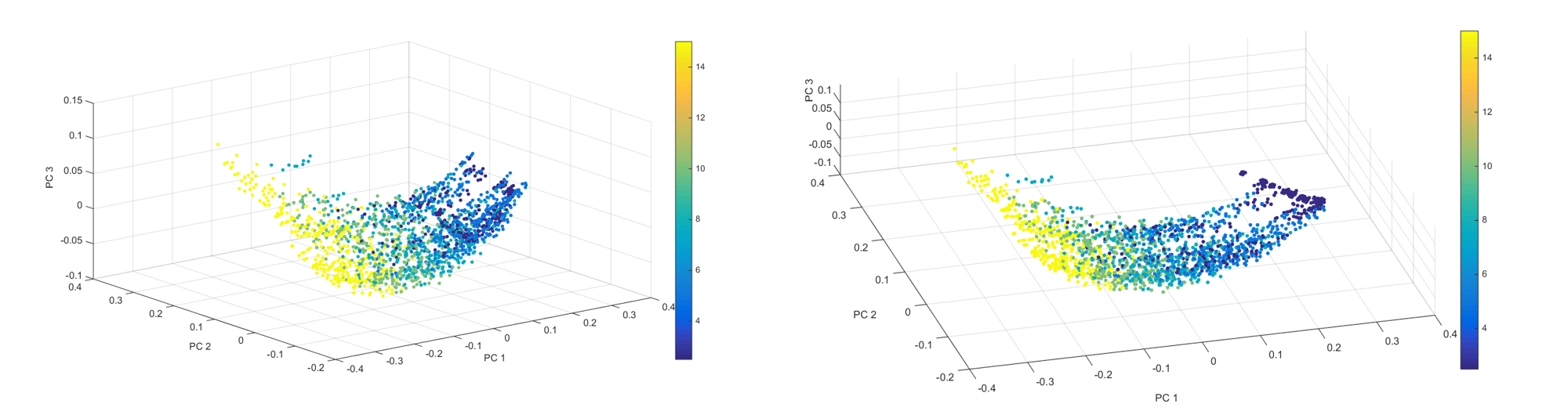 Fig.4. Color coded structures show visual separation in PC space (2 views shown) as a function of V
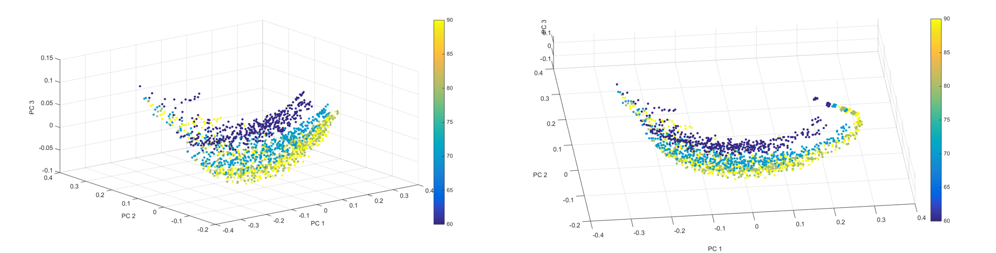 Fig.5. Color coded structures show visual separation in PC space (2 views shown) as a function of W
The V and W parameter-microstructure correlation is displayed as an example but other parameters also display correlation.
Modeling with Polynomial Regression
Modeling the linkages for the entire dataset: Forward method was used to create a model of microstructures a function of the process parameters. Low order polynomial models were used.
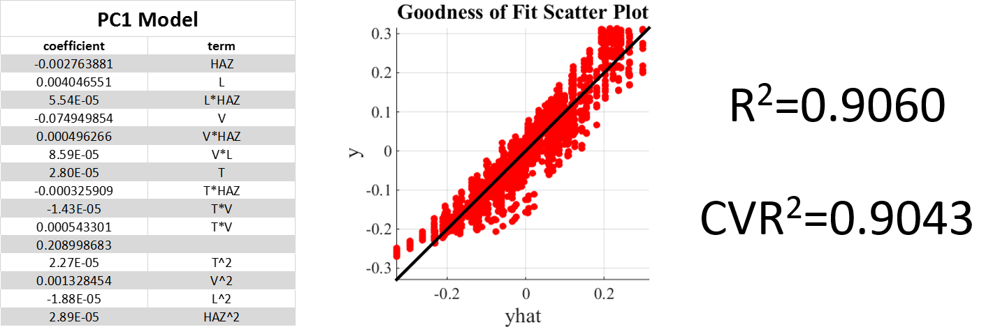 Fig.6. Forward model for PC1 with 4 process parameters and degree 2
Model Improvement
Modeling the entire dataset for CLD structure interpretation should be done with some amount of truncation. The nature of a small subset of the structures makes them ‘low-confidence’ structures as explained here. The models were vastly improved after a truncation of the dataset to structured containing no more than 10% edge chords in the distribution.
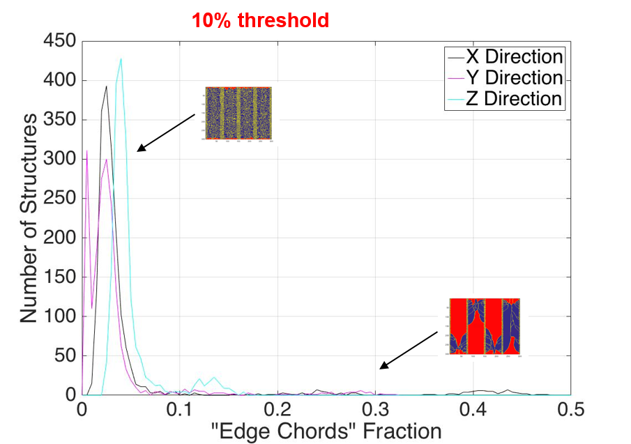 Fig.7. The histogram of the number of structures vs. the edge chord fraction with 10% threshold shown.
The Removed structures are shown below in red and PCA redone on the ‘high-confidence’ dataset.
[discuss the CLD2 thresholding scheme and need for thresholding]
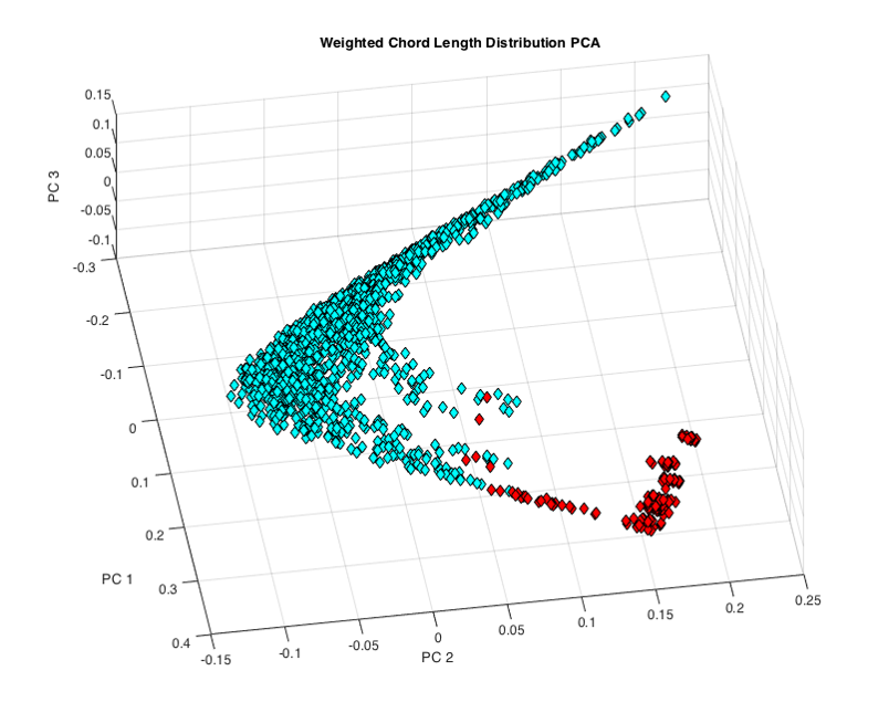 Fig.8. Outliers in the CLD PCA space
The improved model for PC1 is shown below, displaying good fit, low standard deviation and low mean average error.
[discuss the CLD2 thresholding scheme and need for thresholding]
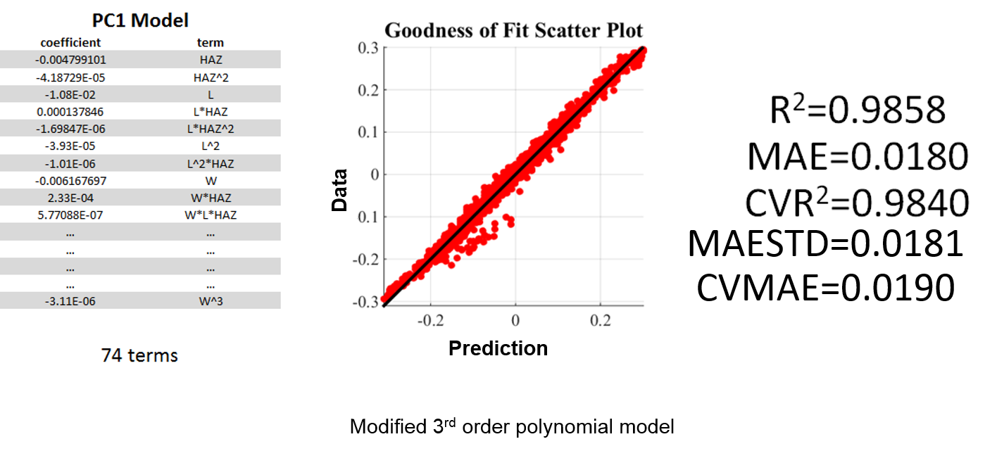 Fig.9. Outliers in the CLD PCA space
The model selection was a comprehensive assessment of R^2 goodnes of fit, Standard deviation, mean average error, and leave one out cross validation CVR^2. Three model classes were defined described by their highest order terms, shown below with the best class shown in red. This class is the modified 3rd order polynomial models.
[fit]
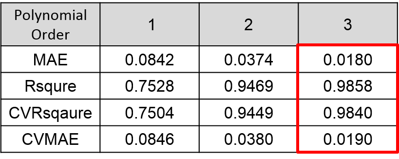 Fig.10. Error analysis among 3 classes of models
Conclusions:
Using data science tools a data-driven model was developed for a LENS-type additive manufacturing system
Process-Structure Linkages were extracted between process parameters and final grain size distributions
Future Work:
- Optimize the data-driven models by exploring other model types and regression types.
- Study the relationship of the truncation threshold on model integrity
- Future work may include the 2pt statistics PCA. The 2-point statistics showed promising results during preliminary tests.
Acknowledgements/References:
- Dr. Surya Kalidindi Ahmet Cecen, Yuksel Yabansu, David Brough, David, Montes, Fred Hohman, Evdokia Popova, Theron Rogers
Presnetation Slides
Process-Structure Linkages in a LENS-type Additive Manufacturing System