Final Post - Grain Growth

This is an executive summary of work done in the Fall 2015 CSE 8803 / ME 8883 Materials Informatics class.

Project members: Fred Hohman, David Montes de Oca Zapiain, and Evdokia Popova

This project builds Structure-Property Linkages for Grain Boundary Pinning during Grain Growth.

Outline

Motivation
Development of our Surrogate Model
Workflow and Data Pipeline
Analysis and Results
Future Work
Acknowledgments

Part I

In this blog post the motivation for the project, the development of the model, the workflow and the results will be addressed and if the reader desired further details, the links to the corresponding posts are provided.

In order to demonstrate the motivation as well as the importance of this project, a brief explanation regarding the grain growth process will be provided.

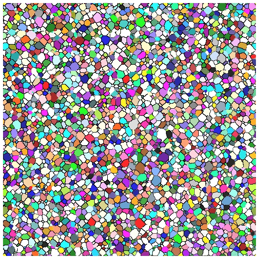
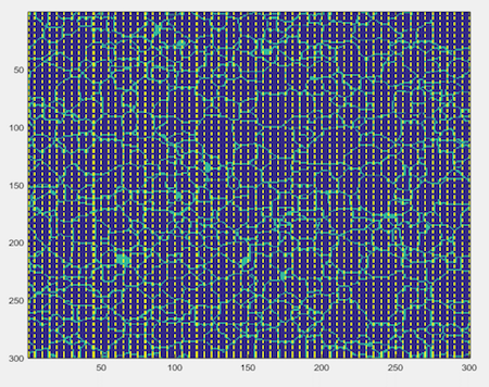
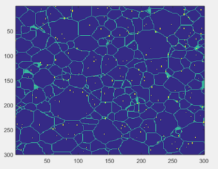
Grain Boundary Pinning is a phenomenon in which insoluble particles are added to a microstructure. These particles affect the final grain size of a microstructure when subjected to a process. It is a common practice in industry to “pin” a material in order to control its final grain size distribution.

These particles are able to affect the grain growth of a microstructure because they reduce the surface area when a grain boundary contacts them. This is important because the driving force of this phenomenon is the grain boundary interfacial free energy.

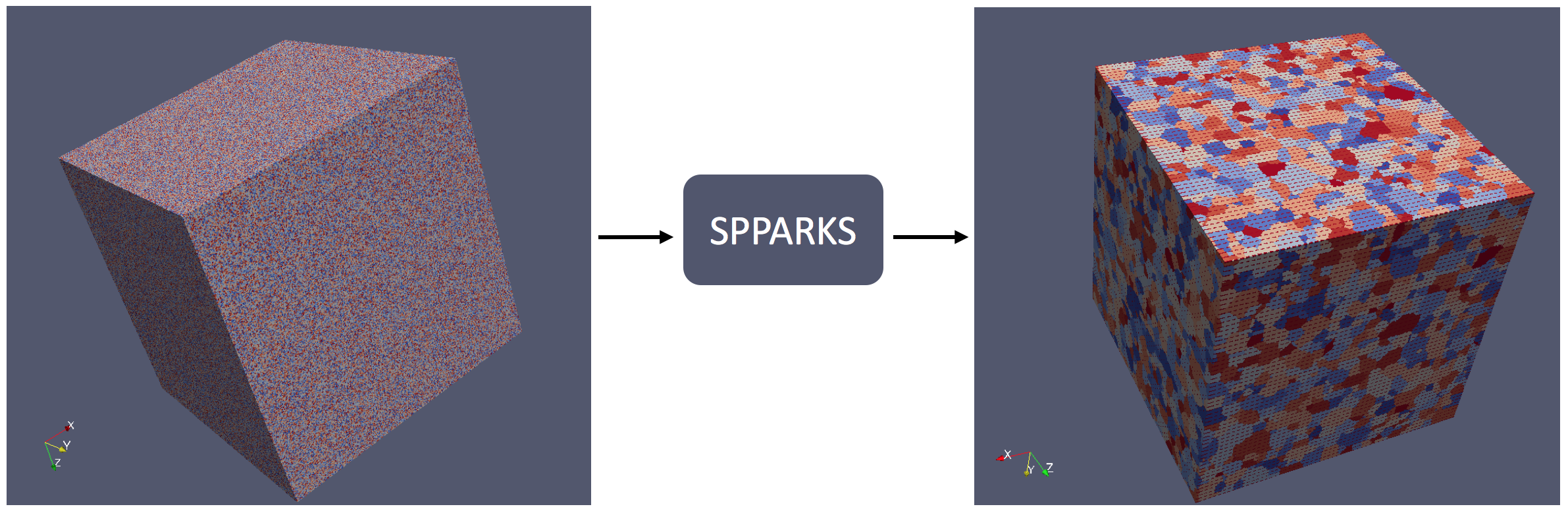
Various tools exist that model this “pinned” grain growth. One commonly used tools is an open source code called SPPARKS (SPPARKS). SPPARKS, developed by (SANDIA national lab), is a code that models pinned grain growth with Kinetic Monte Carlo equations.

Objective

We plan to use a data science approach to build process-structure linkages for grain boundary pinning simulations during grain growth. These linkages will be constructed by first identifying the underlying correlations between an initial distribution of precipitates and the final grain size distribution of the microstructure of interest. Ultimately these linkages will be used to build a surrogate model for SPPARKS.

If further details are desired about pinned grain growth, the objective and the motivation please visit this (post).

Data Generation

The details of the simulations are the following:

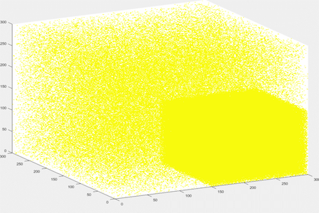
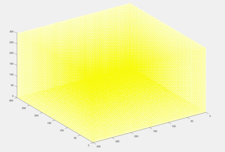
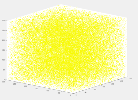
300x300x300 Microstructure
Periodic Boundary Condition
Randomized initial microstructure
20K Monte-Carlo time steps
Constant temperature

In total 220 simulations were performed while varying the following parameters:

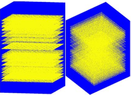
Shape of precipitate: 1, 2, and 3 voxel long precipitates
Volume fraction of precipitates: {.5, 1, 1.5, 2, 2.5, 3}%
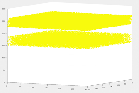
Initial distribution of the precipitates (what we call “classes”)

The simulation pool was built from 5 different initial distributions while varying the above parameters which were defined by us and consulted with SANDIA. The classes defined are believe to encompass a representative space of the possible distributions found in real life. It is important to mention that these pool can be expanded as deemed possible for further use and validation.

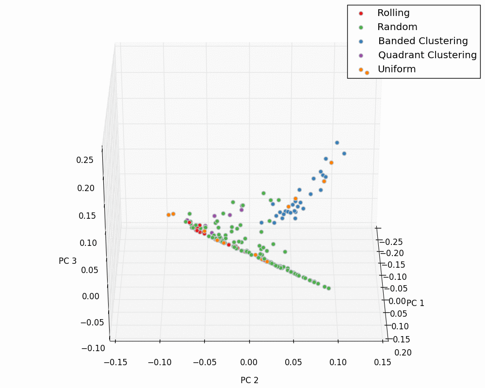
The 5 classes used are the following:

Band Clustering

Quadrant Clustering

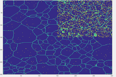
Rolling

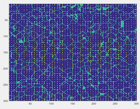
Uniform

Random

Please refer to this (post) for the details on how our data was processed and segmented.

Input and Output of the Surrogate Model

Now that the simulation pool has been built it is necessary to determine the inputs and outputs for the surrogate model to be built.

As mentioned before, the parameters varied within the simulations performed include the shape of the precipitate, the volume fraction of the precipitate, and the distribution of the precipitates, thus it is logical to think that the input for the surrogate model should accurately capture all these variables. The most efficient way to capture these parameters and how they vary is with 2-point statistics, specifically with an autocorrelation of precipitates to precipitates.

The output needs to be identified as well. It is known that the effective property that needs to be extracted from the simulations is the grain size distribution of the final microstructure. Thus it was decided that the best way to acquire this information was to obtain the chord length distribution in the 3 orthogonal directions from the simulation data. This distribution will be used as the output of the surrogate model. It is important to mention that this distribution is also affected by the parameters captured by the defined input for the model, alluding to our claim that the input and output are indeed related (but more on that later!).

For more information regarding the inputs and outputs of the surrogate model please visit the following these posts. (Post 1),(Post 2),(Post 3).

We have now identified inputs and outputs for the surrogate model.

Part II

Our data science approach to building the surrogate models consists of four major steps:

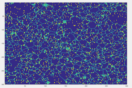
Defining local states: 3-phase material (grains, boundaries, pins)
2-point statistics: autocorrelation of pins
PCA I/O, visualize with 3 components
Model development: linear regression

To see how we carry out each step, consider the following workflow diagram below. Note that each box is considered an “object” (or better yet, some kind of data stored on a computer) and each arrow represents a process or method (a code or script).

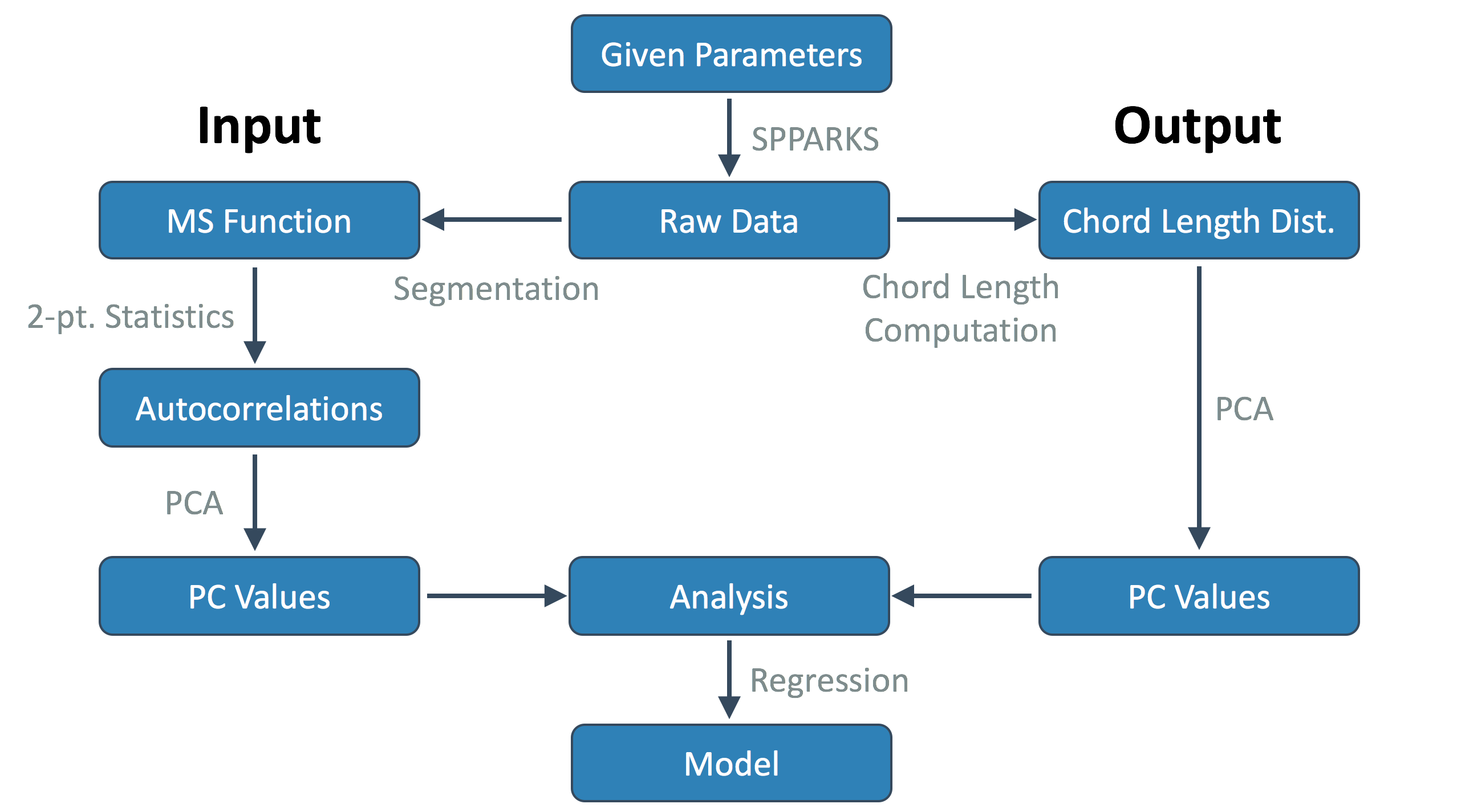
A significant portion of the time spent working on this project was spent creating this data pipeline so that new classes and simulations could be created and funneled through to join the rest of our data. Much of the above pipeline is automated, but we will touch on this at the end of the post.

Results

As we move forward, assume we now have all of our data in a reduced space using PCA. We now will show some sanity checks to make sure our results are correct and make sense.

Confirming Steady State

Recall we are using a code (SPPARKS) to perform our simulations. This code requires a final time-step to terminate at. In order to build a model we need to ensure we ran these simulations long enough, i.e. our pinned microstructure has reached some sort of steady state. To check this, we can consider one simulation from each of our five classes, compute the chord length distribution as time moves forward in the simulation, perform PCA and visual the expected path in PCA space.

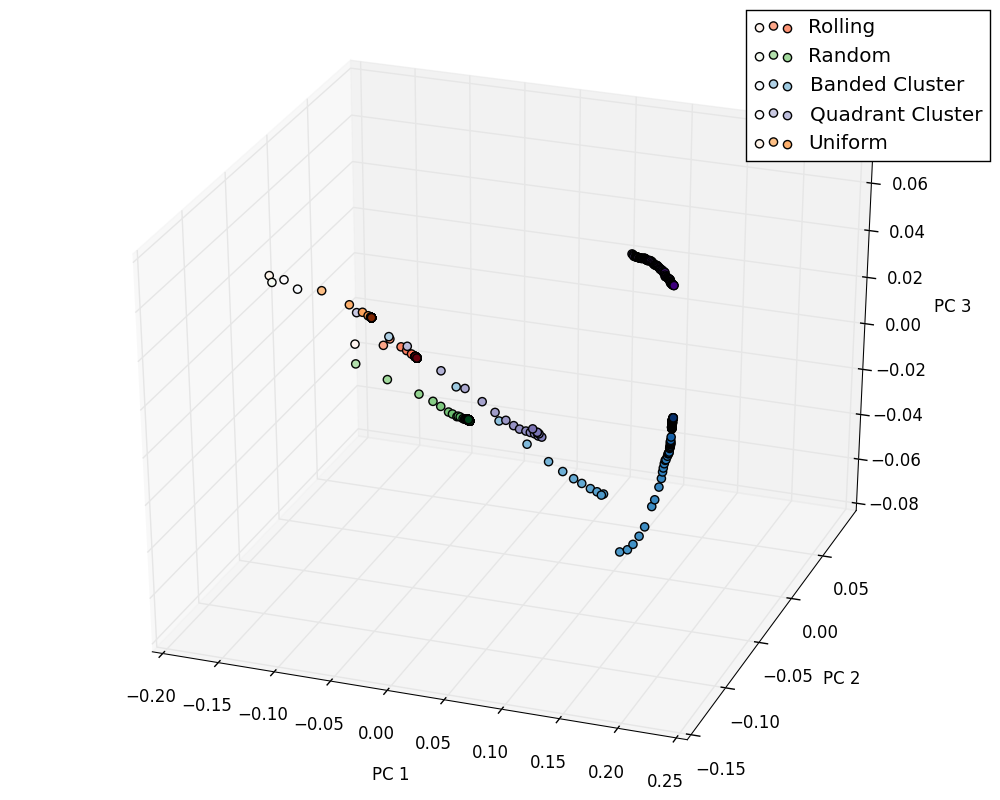
The plot above illustrates this. It shows for each simulation class as time moves forward the color of each point gets darker and closer to the subsequent point, indicating convergence of chord length distribution in simulation-time.

Confirming Output Effects

We also want to check that we chose an input metric (autocorrelations of pins and pins) that correlates to our output (chord length distribution). In a similar qualitative comparison as done above to verify steady state, we will show three simulations chord length distributions evolving in simulation time. These three were chosen from the random distribution class with a fixed percentage, so the differentiating parameter is the shape of the pin, i.e. 1 voxel, 2 voxel, and a 3 voxel long pins.

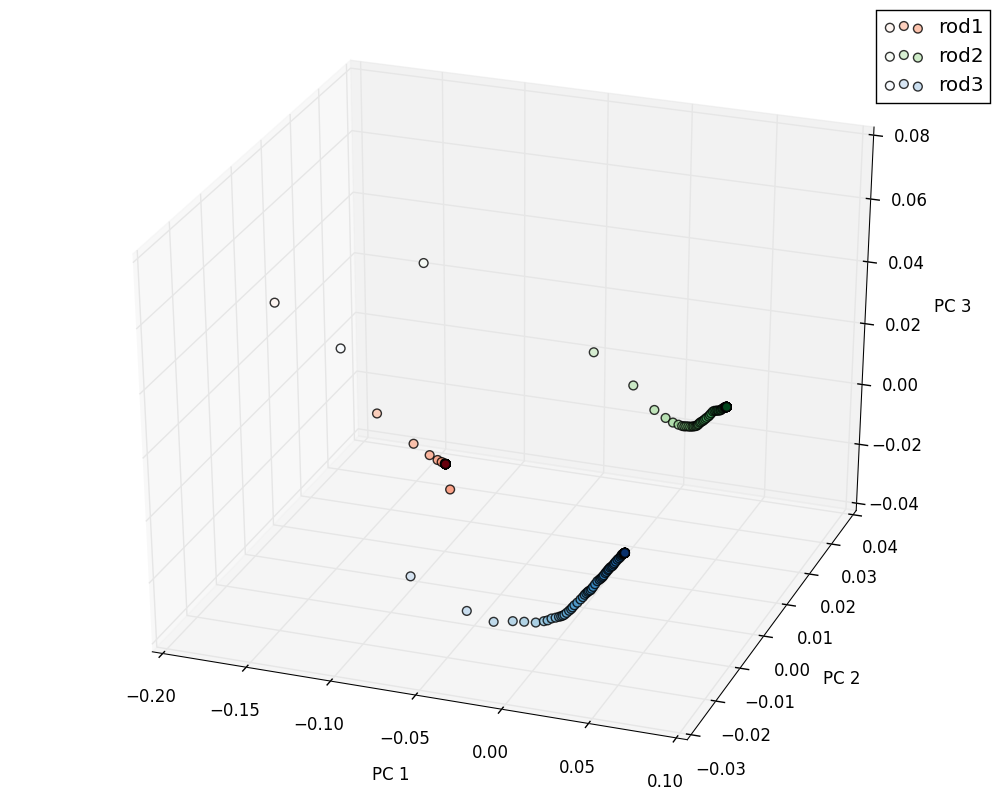
Just as we expected, each simulation convergences to a different point in PCA space which confirms that pin shape does affect grain size.

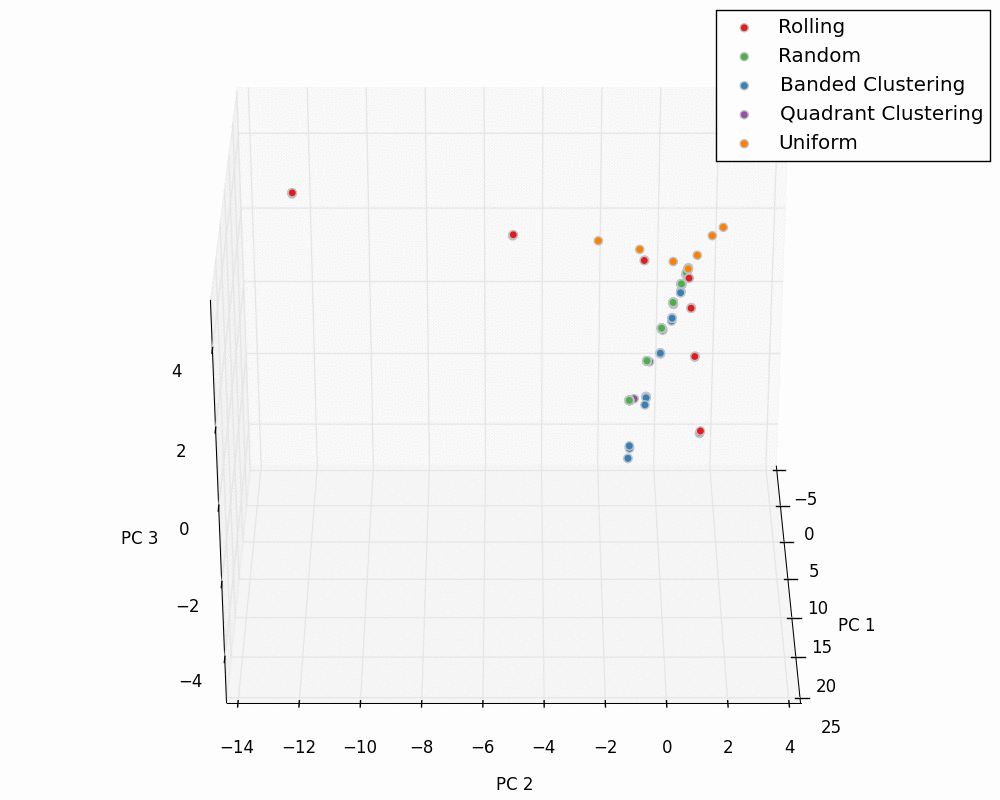
PCA: I/O

We can now plot our entire dataset in PCA space for the input and output PC values. These “master” plots are below.

Input:

Output:

PCA: Scree Plot

To see how well PCA captures the variance of our dataset we can produce scree plots: cumulative percent variance for given amount of PC values.

Input:

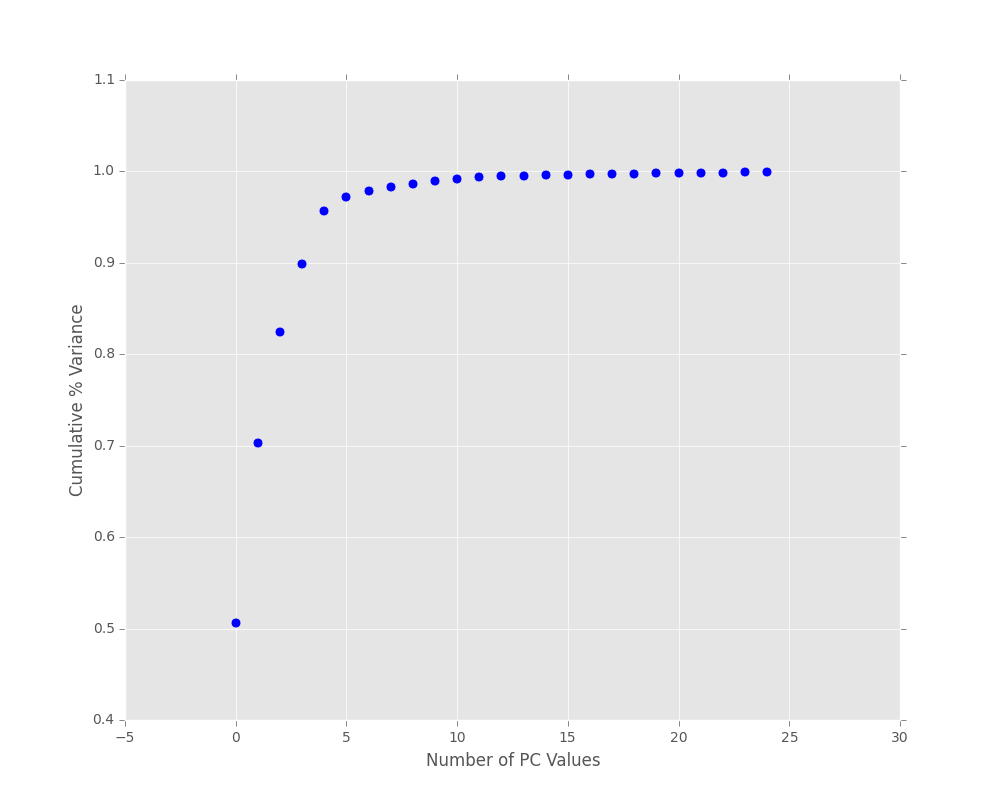
We can see that we are capturing 95% variance in the first 5 PC components.

Output:

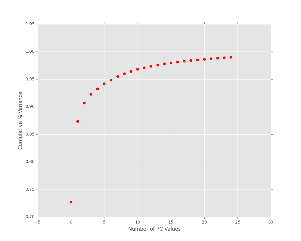
We can see that we are capturing 95% variance in the first 8 PC components.

Regression Results

Now that we have PCA data for our inputs and outputs we can perform regression to build a model between the two and construct a process-structure linkage. To do this we will use Scikit-learn Python implementation of linear regression. We can even optimize the model building procedure to find the best model for a given number of PC values (multiple linear regression) and polynomial degree (multivariate regression). We broke our data up into two pieces: 80% to use as training data, and the remainder 20% to use as test data. We then performed leave-one-out cross-validation methods to obtain mean squared error for each model. We did this for high combinations of PC values and polynomial degree and found the point at which we began to see over-fitting affect our MSE value.

From the code we receive the following output:

Order of Polynomial: 1, Number of Components: 10, MSE Value: -2.70392576062e-05

This shows our best model to build a process-structure linkage is a linear model using 10 PC components.

Conclusion

With the data we have generated through the semester we were able to use novel data science tools to develop a surrogate model for grain boundary pinning during grain growth simulations. More importantly, our work done establishes a material informatics framework that is generalized, automated, and scalable which can be extended to other models.

Future Work

Our project encompassed data generation, simulations, material informatics problem solving, and analysis, however due to the amount of time in a semester we were not able to finish everything we initially sought. To improve our project we would like to:

Evaluate our current dataset relevance to physical materials.
- This includes expanding our simulation pool to include more representative data.
Expand the model capabilities and predictions for newly generate data.
Further model validation, such as testing limiting cases.

Acknowledgments

We would like to first thank Dr. Surya Kalidindi for his expertise and guidance. We also would like to thank David Brough and Ahmet Cecen for their help in workflow development. Finally, we would like to thank Dr. John Mitchell (Sandia national labs) for his suggestions and comments on our project while we were still generating data.

References

Gladman, T. (1966). On the theory of the Effect of Precipitate Particles on Grain Growth in Metals. Proceedings of the Royal Society of London.Series A, Mathematical and Physical Sciences (294), 298-309.
Hillert, M. (1965). On the theory of normal and abnormal grain growth. Acta Metallurgica , 13, 227-238.
Kalidindi, S. (2015). Hierarchical Materials Informatics. Oxford: Elsevier.
Plimpton, S., Battaile, C., Chandross, M., Holm, L., Zhou, X., & al., e. (2009). Crossing the Mesoscale No-Man’s Land via Parallel Kinetic Monte Carlo. Sandia report.
SANDIA National Lab. (2009). SPPARKS Kinetic Monte Carlo Simulator. http://spparks.sandia.gov/index.html
Wheeler, Daniel; Brough, David; Fast, Tony; Kalidindi, Surya; Reid, Andrew (2014): PyMKS: Materials Knowledge System in Python. figshare. http://dx.doi.org/10.6084/m9.figshare.1015761

Final Thoughts

As we worked on this project certain components underwent changes in research direction, so some of the older blog posts may not reflect the final content present above (or may even be irrelevant). If you have any questions regarding a specific component feel free to contact any one of the project members: