Project Intro
This project centers around the time evolution of an active nematic material on the surface of a torus. We define an active material as a material whose individual components have a source of internal energy that is converted into kinetic energy. Nematic materials are an ordered material composed of elongated units who share a preferred alignment direction. We refer to this direction as the director, n. In equilibruim with no external perturbation, a nematic material will have a uniformly aligned ground state; however, external influences such as confinement, applied fields, flow, etc can produce states with defects, or places where the n is undefined. A schematic of how a director is defined as well as director maps of two differnt defect types can be seen in the figure from the Introduction Post can be seen below.
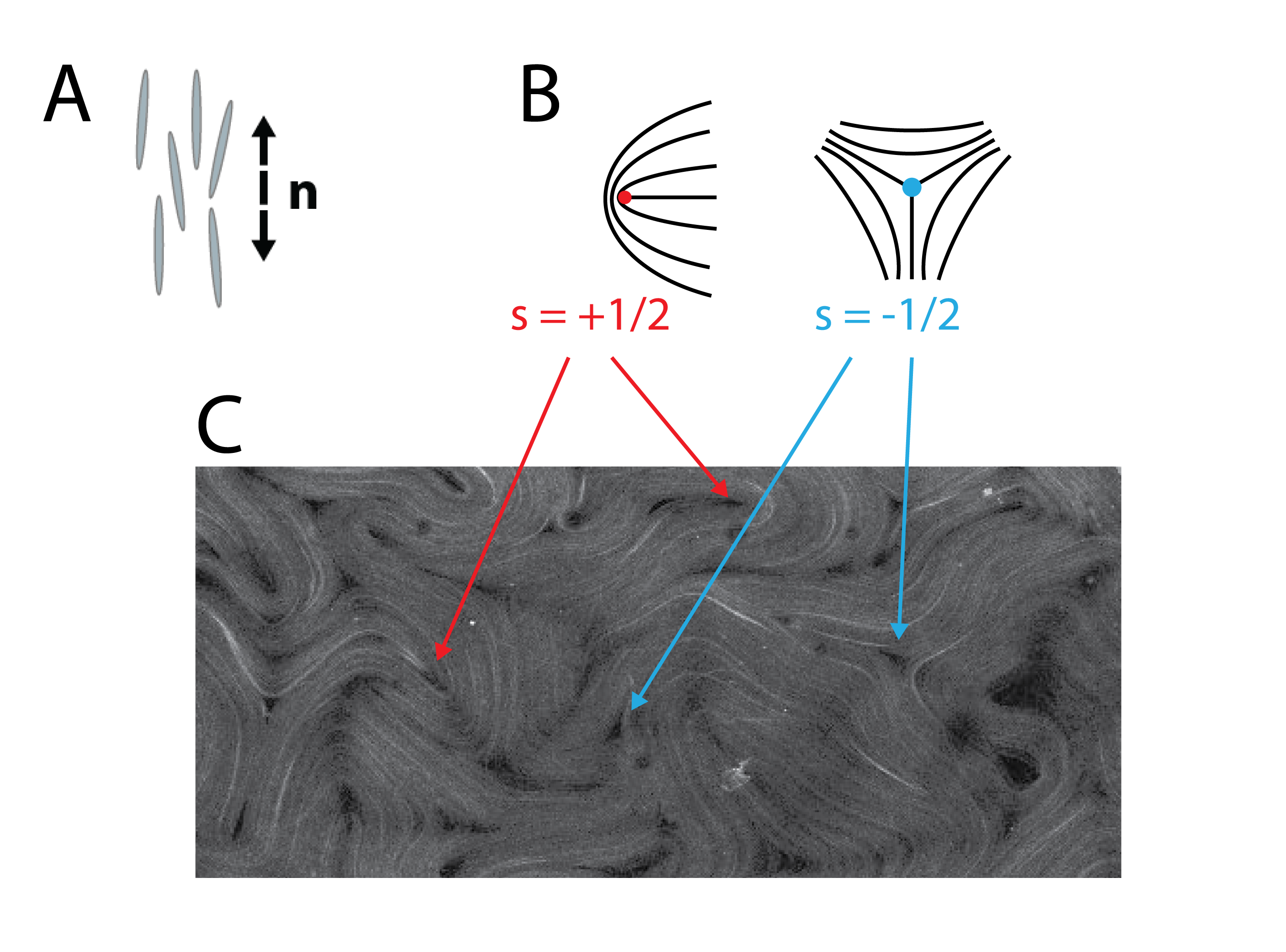
Active nematics present an interesting way to examine ordered materials that are constantly driven out-of-equilibrium. A snapshot of an active nematic can be seen in the figure above. Note the large number of and defects in the sample. This is due to activity-induced flow distorting the preferred uniform ground state. More about the specific active nematic system we use and some of its fundamental science applications can be found here and here. Specifically, we wish to look at active nematics on the surface of a torus; there are many connections between equilibrium nematics and topology/curvature. For example, this study looking at equilibrium spherical nematic shells and this study looking at bulk equilibrium nematic toroids. As seen here, active nematic spheres have been studied and a correspondence was found between the active case and the equilibrium case. We hope that studying active nematics on a torus will lead to insights not only concenrning the equilibrium ground state of a nematic on a torus, but will also lead to insights in non-equilibrium physics.
To do this, we start with the goal of characterizing the time-evolution of the structure of the active nematic on the surface of a torus.
The Dataset
Our data are collected with a confocal microscope; thus, we have intensity data in a 3-D (x,y,z) array. Below left is a scan of an example array through the z-direction, and below right is a video rotating the array to show that we do have a nematic on the surface of a torus.
|
z-stack |
reconstructed image |
Both of these images come from the same dataset - it is a single image in time of a single torus. For the time-evolution data, we are going to project the data along the z-axis to form a 2-D image (x,y). A video of the time evolution of such a projection for a small portion of the the torus is below.
|
example active nematic data |
The above video is one of the datasets we wish to charaacterize. We have 2 other videos like the above video, but for different toroids with different sizes and aspect ratios. More info can be found in the Introduction Post.
Cleaning the images
To track the time-evolution of the structure, we first need a way to characterize the structure. We do this using the tensor nematic order parameter Q, as defined in this post. Since Q is a tensor, we need 2 quantities to define the structure at every point. We will use the n as defined earlier and “S”, the degree of alignment. A more in-depth description as well as our methodology for determining n and “S” from the raw data can be found in this post. Once the images are clean, we have an n image and an “S” image for each raw data image, as seen in the example below:
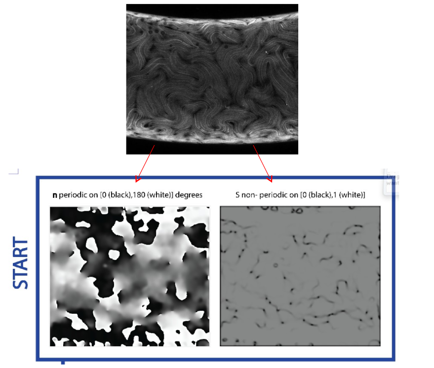
The n image shows the orientation of the director on the interval [0 degrees, 180 degrees] measured clockwise off of the horizontal axis. The “S” image holds the degree of alignment and can take values from [0,1].
The next step to cleaning the images is to unwrap them; since we have projected a curved surface in 3-D to a flat 2-D plane, distance is no accurately represented in the projections. This will be a problem for computing statistics. Thus, we will “unwrap” our projected images such that the area on the surface of the torus is preserved in the 2-D plane. An example unwrapping can be seen in the below image.
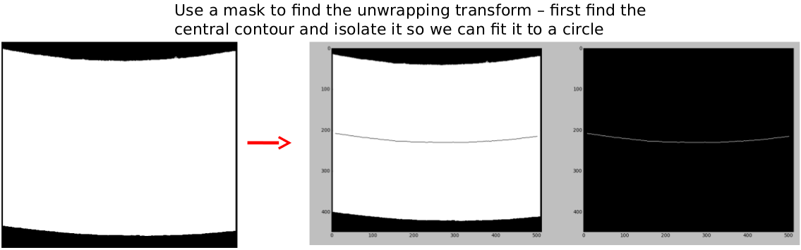
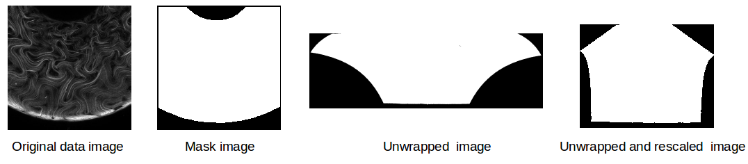
The highlighed contours and colored endpoints correspond to each other. Note how even though we’ve unwrapped one curvature, we haven’t yet projected length properly. The schematic above just serves as a useful graphic to demonstrate part of the unwrapping process. Our final process rescales the unwrapped image to properly represent data, as seen below for a series of binary mask images.
More about the unwrapping process can be found here.
Workflow
Now that our images are clean, we need to construct a processing pipeline to characterize the time evolution of the structure. This pipeline can be seen here. In short, it reads something like: Clean images -> statistics -> dimensionality reduction via PCA -> model.
Challenges
We spent a large part of this semester trying to work out some of the issues with the pipeline. Specifically, we got hung up on:
What should we look at?
Unlike many systems that have already been treated with PyMKS and MatIN, we believe that spatial position in the sample matters. One of the defining features of a tirus is the fact that the Gaussian curvature varies from politive along the outer ring of the torus to negative along the inner ring of the torus. As curvature has been shown to have an effect on ordered materials (especially nematic ordered materials), we expect that the position of the nematic on the turs will affect its structure. To deal with this without keeping independent statistics for every point, we decided to try and bin the images by their Gaussian curvature - in this way we should be able to see if different bins have different structure. More on the binning can be found here.
One of the issues with this approach is that the bins can be small; since the size of the statistics images passed to PCA must be the same, we are limited by our smallest bin. As this could cause problems, we will also try analyzing the whole torus (as if spatial position is irrelevant) as a comparison. See post 9 for more details concenring the unbinned stats.
Implementing the Fourier Basis
Another unique aspect of this system is that n is periodic, which requires a periodic basis function to accurately represent. We use the Fourier series, defined here to discretize n. Examples of oiur data properly discretized can be seen here.
How many terms in the Fourier Series should we use?
Apart from the challenges of implementing the Fourier series (see here for an early attempt where the implementation of the Fourier series was still wrong), there is the cahllange of determining the optimal number of components in the Fourier series to use to best represent the microstructure. From a resources standpoint, anything more than 9 terms in the Fourier series is is too large for even the PACE cluster to handle. However, as seen in the plot below of variance by PCA component for different numbers of terms in the Fourier series, the data aren’t very well represented with only 9 Fourier components.
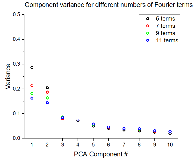
The above plot was run on a small subset of images, so we were able to look at 11 terms in the Fourier series. When running on all the data we have issues with anything more than 9 terms. More on this issue can be found in these two posts (1) (2). This is still an ongoing issue, but we decided to run PCA on what we could just to see if we were able to get meaningful results even if the captured variance is low.
Preliminary results
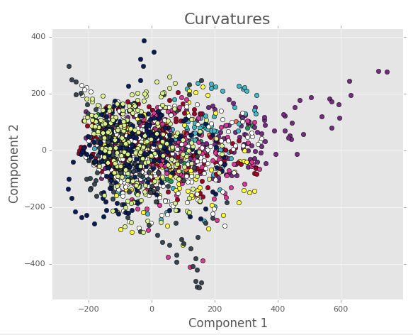
First, looking at the PCA for the binned images, it’s easy to see that all the data are clustered together in a big mass. All the images can be found here, but an example image for PCA components 1 and 2 is seen below.
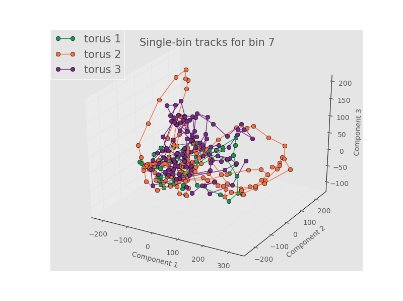
Even when we look at an individual bins and connect the points to highlight the time evolution we don’t see any meaningful separattion. Bin 7 (0 to slighly positive Gaussian curvature) and PCA components 1-3 is shown below. The rest of the tracks are foundhere
Here we are left with the conclusions that either (1) we don’t have enough terms in the Fourier series, (2) the spatial position doens’t really matter, (3) there’s no meaningful variation between samples, or (4) the linear dimnensionality reduction of PCA is unsuited for a nonlinear process like this one. Some of these concerns are addressed by looking at the results from the full, unbinned images. An example for the first 3 PCA components is below.
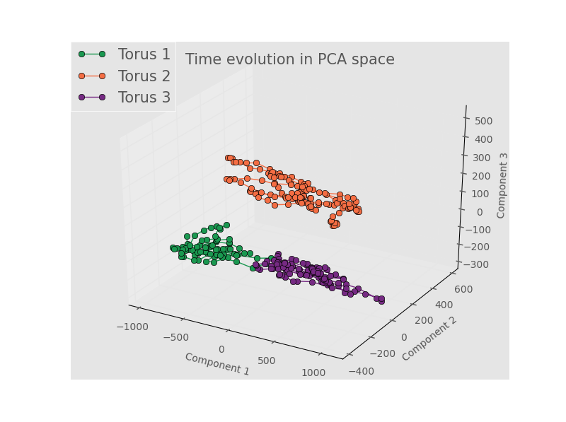
The rest of the images can be found here. Note that there is some separation in the 1st three components, and that the structure for each torus seems to evolve in small regions of PCA space.
Conclusions
We didn’t have quite enough time to develop a model for the structure evolution this semester, but this project will continue into the Spring, so we still have more time. In addition, we would like to take a closer look at our binning process to see if we can be more conclusive if spatial position matters when determining the structure for this system. Overall, we have a good start in characterizing the time evolution of the structure of the active nematics, but more needs to be done to truly understand the physics at play.